Regrid options

This document provides in-depth explanation for the main options of regrid().

Input definition

Input data may be specified either by giving a path in the Source parameter or by giving a GRIB-based data object in the Data parameter. Note that you should specify either Source or Data, not both.

Source: path to a GRIB file
Data: GRIB-based data object

Drop a MARS Retrieval or a GRIB file icon inside this icon field. In Python or Macro, supply a Fieldset object.

Output definition

Grid Definition Mode

Select a method for specifying the output grid.

Grid: supply a valid string or list of numbers in the Grid parameter
Lambert Conformal or Lambert Azimuthal Equal Area: supply details of the output grid in the set of Lambert grid definition parameters
Template: supply a template whose grid structure will be used to generate the output GRIB
- Note 1: use either Template Source or Template Data to specify the template (not both)
- Note 2: only GRIB fields on regular lat/lon or regular/reduced Gaussian grids may currently be used as templates
Filter: in this mode, the output grid will be the same as the input grid, with interpolation acting as a filter
- Note 1: this is equivalent to Template, with the input serving as the template (same input format limitations apply)
- Note 2: Interpolation as k-nearest neighbours is the only method able to support filtering

Grid

Supply a grid definition as described here: grid - keyword in MARS/Dissemination request.

Examples of valid grid definitions:

GUI	Python / Macro	Result
1/1	[1, 1] or “1/1’”	A regular lat/lon grid with 1x1 degree point spacing
0.2 5/0.25	[0.25, 0.25] or ” 0.25/0.25”	A regular lat/lon grid with 0.25x0.25 degree point spacing
O1280	“O1280”	An octahedral reduced Gaussian grid, octahedral with 1280 latitude lines between the pole and equator
N640	“N640”	An ‘original’ reduced Gaussian grid, with 640 latitude lines between the pole and equator
F400	“F400”	A regular Gaussian grid, with 400 latitude lines between the pole and equator

This parameter can be left empty to preserve the grid properties (regular/reduced lat/lon or Gaussian) while performing other kinds of post-processing (changing bits per value, calculation of gradients, etc.).

Template Source

If Grid Definition Mode is Template, set path to a GRIB file to be used as template.

Template Data

If Grid Definition Mode is Template, set a GRIB-based data object to be used as template.

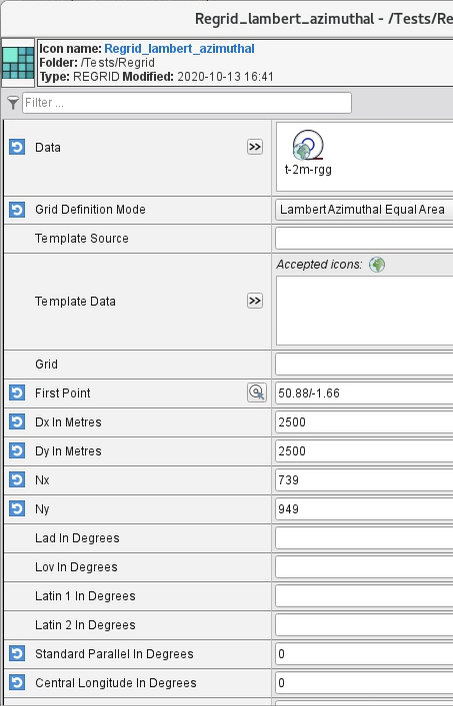
Lambert Conformal or Lambert Azimuthal Equal Area parameters

These projections require setting several parameters, named following the convention in their descriptions:

Lambert Conformal (see GRIB template here)
Lambert Azimuthal Equal Area (see GRIB template here)

Most of these parameters are required and do not have default values, meaning that they must be filled in. The parameters are:

First Point: defines the North/West (or top/left) point in the unprojected frame (lat/lon)
Dx In Metres: x-direction increment in the projected frame (x/y)
Dy In Metres: y-direction …
Nx: number of points along x-direction in the projected frame (x/y)
Ny: number of points along y-direction …
Specific to Lambert Conformal:
- LaD In Degrees
- LoV In Degrees
- Latin 1 In Degrees (defaults to LaD In Degrees)
- Latin 2 In Degrees **(defaults to **LaD In Degrees)
Specific to Lambert Azimuthal Equal Area:
Standard Parallel In Degrees
Central Longitude In Degrees

Here are examples of generating Lambert grids.

Example

Lambert conformal

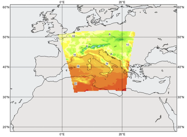
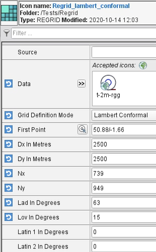
regrid_lambert_conformal = mv.regrid(
   grid_definition_mode = "lambert_conformal",
   first_point          = [50.88,-1.66],
   dx_in_metres         = 2500,
   dy_in_metres         = 2500,
   nx                   = 739,
   ny                   = 949,
   lad_in_degrees       = 63,
   lov_in_degrees       = 15,
   data                 = t_2m_rgg
         )

Example

Lambert_azimuthal equal area

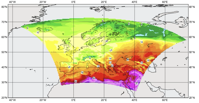
regrid_laea = mv.regrid(
   grid_definition_mode         = "lambert_azimuthal_equal_area",
   first_point                  = [66.982143,-35.034024],
   dx_in_metres                 = 5000,
   dy_in_metres                 = 5000,
   nx                           = 1000,
   ny                           = 950,
   standard_parallel_in_degrees = 52,
   central_longitude_in_degrees = 10,
   data                         = t_2m_rgg
   )

Wind processing

Activates processing that is particular to wind fields. Winds are represented by its vector Cartesian components u/v (gridded) or U/V (spectral) and, typically, they are archived as (spectral) vorticity/divergence (vo/d.) The relation between the spectral and gridded wind components is u = U / cos(latitude) and v = V / cos(latitude).

It is up to the user to specify if the input consists of wind fields. Set this appropriatelly in order to perform the correct processing.

Possible options are:

U/V to u/v	Converts pairs of Cartesian components vector fields (spectral) U/V to (gridded) u/v. This option is required if regridding wind fields on/to a rotated grid. Note: assumes that the input come in pairs of alternating U/V.
vo/d to u/v	Converts pairs of (spectral) vo/d fields into (spectral) U/V or (gridded) u/v. In case of gridded output, scaling by the cosine of their latitudes is applied (as above.). Note: assumes that the input come in pairs of alternating vo/d.
Off (default)	Each processed field is treated individually.

Spectral to grid inverse transform

If the input files are spectral, the following parameters are used to fine-tune the conversion to grid points. The general workflow is:

spectral data (input)
if Truncation is not None (default Automatic), spectral data is truncated (intermediate spectral field, controlled by Truncation)
if Intgrid is not None,
1. inverse transform produces an (intermediate gridded field, controlled by Intgrid),
2. interpolation to (final) grid
if Intgrid is None, inverse transform produces the (final) grid

Note: if the intended (final) grid is rotated, or a given projection (eg. Lambert Conformal, LAEA, etc.), is very expensive computationally
final gridded data (see Grid Definition Mode)

Truncation

Spherical harmonics truncation, as described here: truncation - keyword in MARS/Dissemination request.

When the output is spectral, defines the output intended truncation; When the output is gridded, defines the intermediate truncation before spectral inverse transform to gridded space. Possible values are Automatic, None or a number describing the spectral truncation to be applied.

Intgrid

Intermediate grid when performing spectral inverse transform to gridded space, as described intgrid - keyword in MARS/Dissemination request.

Possible values are:

Automatic: regular Gaussian grid, with N given as linear spectral order relation to output grid latitude increments
Source: octahedral reduced Gaussian grid, with N given as cubic spectral order relation to output grid latitude increments (mimics dissemination)
None: no intermediate grid, spectral inverse transform target is the user’s intended output (costly if many different outputs are intended)
name of the desired intermediate grid

Interpolation methods and parameters

There is a high degree of customisation available to parametrise the available interpolation methods. Please note:

Not all the interpolation methods support all possible grid types
Even though the editor tries to avoid these, some inconsistent option combinations are allowed

Interpolation

Specifies the type of interpolation to be used on the fields. The default is Automatic, which selects either Linear or Nearest Neighbour based on an internal table of known parameters. If the parameter is unknown, the default will be Linear. The possible interpolation methods are:

Finite Element-based interpolation with linear base functions
- Linear: FEM with supporting triangular mesh
- Bilinear: FEM with supporting quadrilateral mesh (for reduced grids, possibly containing triangles instead of highly-distorted quadrilaterals)
Grid box method (based on Model grid box and time step)
- Grid Box Average: input/output grid box intersections interpolation preserving input value integrals (conservative interpolation)
- Grid Box Statistics: input/output grid box intersections value statistics - see parameter Interpolation Statistics for possible computations
K-nearest neighbours based:
- K-Nearest Neighbours: general method combining nearest method (choice of neighbours) and distance weighting (choice of interpolating neighbour values)
- Nearest Neighbour: parametrised version of K-Nearest Neighbours to chose a nearest neighbouring input point to define output point value
- Nearest LSM: interpolated output point takes input only from input points of the same type (land or sea — requires setting land/sea masks)
Structured methods, exploiting grid structure and configurable stencil for fast interpolations (non cacheable, so do not benefit from speedups on subsequent runs)
- Structured Bilinear: bilinear interpolation
- Structured Bicubic: bicubic interpolation
- Structured Biquasicubic: computationally economic bicubic interpolation
Automatic: see above.

Nearest Method

Available for any of the ‘nearest’ interpolation methods; Supports Interpolation K-Nearest Neighbours or Nearest LSM. Possible values are:

Distance	input points with radius (option Distance) of output point
Nclosest	n-closest input points (option Nclosest) to output point (default 4)
Distance and nclosest	input points respecting Distance ∩ Nclosest
Distance or nclosest	input points respecting Distance U Nclosest
Nclosest or nearest	n-closest input points (option Nclosest), if all are at the same distance (within option Distance Tolerance) return all points within that distance (robust interpolation of pole values)
Nearest neighbour with lowest index	nearest input point, if at the same distance to other points (option Nclosest) chosen by lowest index
Sample	Sample of n-closest points (option Nclosest) out of input points with radius (option Distance) of output point, not sorted by distance
Sorted sample	as above, sorted by distance

Associated options supporting Grid Box Statistics (described above):

Distance: in [m] choice of closest points by distance to input point
Distance Tolerance: in [m] tolerance checking the farthest from nearest points (when Nearest Method is Nclosest or nearest)
Nclosest: choice of n-closest input points to input point

Interpolation Statistics

Associated options supporting Nearest Method (described above). Possible values are:

count
count_above_upper_limit
count_below_lower_limit
maximum
minimum
mode_real
mode_integral
mode_boolean
median_integral
median_boolean
mean
variance
skewness
kurtosis
stddev
automatic

Distance Weighting

Only available if Interpolation is K Nearest Neighbours. General way on how to interpolate input neighbouring point values to output points, including the Inverse Distance Weighting (IDW) class methods (see Wikipedia), which operates over input points returned by Nearest Method. Possible values are:

Climate Filter	filter for processing topographic data (see IFS documentation, Part IV: Physical Processes,11.3.1 Smoothing operator)
Inverse Distance Weighting	IDW of the form \(distance^{-1}\); If input points match output point, only that point’s value is used for output
Inverse Distance Weighting Squared	IDW of the form \((1 + distance^{2})^{-1}\)
Shepard	DW of the form \(distance^{-p}\) (option Distance Weighting Shepard Power, default 2.)
Gaussian	IDW of the form \(exp(\frac{-distance^{2}}{2\sigma^{2}})\) (option Distance Weighting Gaussian Stddev, default 1.)
Nearest Neighbour	emulate Interpolation as Nearest Neighbour by picking first point (note that, when Nearest Method is Sample, a random near point is picked)
No	no distance weighting, average input values (irrespective of distance)

On multiple input points, weights are normalised linearly to unity. Associated options supporting Distance Weighting (described above):

Distance Weighting Shepard Power: specify Shepard’s method power parameter (see Wikipedia specific section)
Distance Weighting Gaussian Stddev: specify Gaussian standard deviation (see Wikipedia)

Non Linear

This treatment is applied after calculation of the interpolation weights, and before they are applied to input values to generate output values. This allows modifications of these weights based on input data, such as the presence of missing values — In any case, no missing values are ever used for interpolation.

Most of the options avaiable concern modyfing the set of input points weights pertaining to a specific output point. When removing interpolation weights (pe. because they point to a missing value) all the remaining interpolation weights are re-normalised (linearly) to sum(wi) = 1.

Possible values are:

Missing If All Missing	if all input point values (contributing to an output point) are missing, set output value to missing (it requires all input point values to be missing)
Missing If Any Missing	if any input point values (contributing to an output point) are missing, set output value to missing (it suffices one input missing value)
Missing If Heaviest Missing (default)	if the most significant point for interpolation (largest interpolation weight) is missing, set output value to missing (typically, not generally, this corresponds to the nearest input point)
Simulated Missing Value	allows a user-specified value (option Simulated Missing Value) with a tolerance (option Simulated Missing Value Epsilon). In the presence of missing values this can can create wrong results.
Heaviest	emulate Interpolation as Nearest Neighbour by selecting the most significant point for interpolation to each output point (discarding the other contributions)
No	no non-linear corrections are applied. In the presence of missing values this can can create wrong results.

Associated options supporting Non Linear (described above):

Simulated Missing Value: if Non Linear is Simulated Missing Value, set which value should not be used for interpolation irrespective of how data is described
Simulated Missing Value Epsilon: if Non Linear is Simulated Missing Value, set tolerance when checking for value not be used for interpolation

Land-sea mask parameters

Land-sea masks (LSMs) can be configured for two different purposes:

when Interpolation is Nearest LSM: use input/output LSMs to distinguish between points used for interpolation; If output point is land, only input points on land are used for interpolation (respectivelly for sea points)
when Interpolation is not Nearest LSM and LSM is On (as described here: lsm - keyword in MARS/Dissemination request): interpolation weights for input points are rebalanced (by factor LSM Weight Adjustment) if output point is of different type to input points; Results depend strongly on interpolation method (in addition to the LSM parameters)

Distance Weighting With LSM

Only available if Interpolation is Nearest LSM. Possible values are:

Nearest LSM: chose the closest input point (no disambiguation if there is more than one closest point at the same distance)
Nearest LSM With Lowest Index: cross-platform compatible version (of the above Nearest LSM) with disambiguation of closest input points at the same distance of output points
Off: use internal defaults (currently set to Nearest LSM With Lowest Index)

LSM Weight Adjustment

Only available if LSM is On, this is the factor adjusting input point weights if they are not of the same type (land/sea) as related output point; On application, all contributing input point weights are re-normalised (linearly) to sum(wi) = 1.

LSM Selection Input/Output

Specifies whether the input/output LSM file will come from LSM Named Input/Output (named, default) or LSM File Input/Output (file).

LSM Named Input/Output

Select one of the predefined names from the following:

1km (default)	binary-based LSM sourced from MODIS Land Water Mask MOD44W (see referene)
10min	binary-based LSM at high resolution (legacy, pre-climate files version 15)
O1280	GRIB-based IFS supporting climate files version 15, on this specific grid
O640	(as above, for this grid)
O320	(as above, for this grid)
N320	(as above, for this grid)
N256	(as above, for this grid)
N128	(as above, for this grid)

LSM File Input/Output

Provide the path to an input/output LSM GRIB file.

LSM Interpolation Input/Output

If input/output is not on the same grid (geometry) as provided input/output LSM (respectively), interpolate with this method to a temporary LSM with required geometry.

LSM Value Threshold Input/Output

For GRIB-based LSM (so excluding ‘1km’ and ‘10min’), the threshold for condition (value ≥ threshold) to distinguish land (true) from sea (false).

Nabla differential operators

This options allows application of differential operators to input fields. The current available approach is similar as used in the Finite Volume Module of the IFS, specifically:

It employs an edge-based, median-dual finite-volume method, with field values interpreted as averaged quantities of the supporting “dual cells”.

There is support for both scalar and vector (u/v) fields; Due to the geometrical interpretation being ill-posed at the poles (singularities) there is an additional option to force missing values at the poles.

Nabla

Activates a nabla (differential) operator processing on the fields. Possible options are:

Scalar Gradient	Scalar field gradient (∇)
Scalar Laplaciant	Scalar field Laplacian (∇²)
UV Gradient	Vector (u/v) field gradient (∇)
UV Divergence	Vector (u/v) field divergence (∇⋅)
UV Vorticity	Vector (u/v) field vorticity or curl (∇×)
Off (default)	no differential processing

Nabla Poles Missing Values

Due to the supporting differential operators calculation method, values aren’t well defined at the poles (singularities); This option allows forcing missing value at the poles. Possible values are On and Off.

Extra Processing

Area

Supply a grid definition as described here: area - keyword in MARS/Dissemination request (swapping north/south).

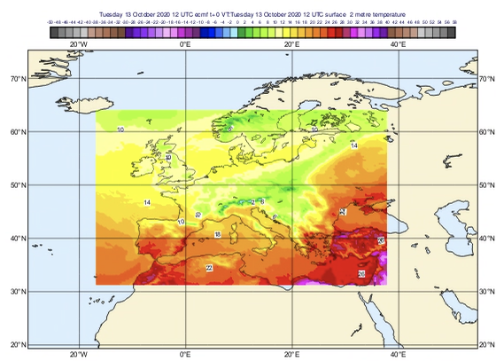
Specifies the geographical area that the output fields will cover, the default being for the whole globe. Enter lat/lon in degree bounds of an area separated by a “/” (south/west/north/east), or in Macro or Python provide a list, e.g. [south, west, north, east]; alternatively, use the assist button to define the area graphically.

For example, this set of parameters generates the following output data:

t01 = mv.regrid(
   grid     = [0.1,0.1],
   area     = [31,-17,64,38],
   data     = t_2m
   )

mv.plot(t01)

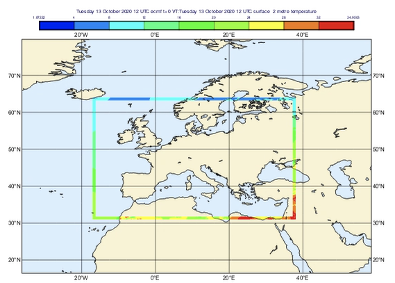
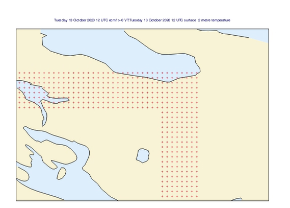
Frame

Specifies the width of a frame within a given sub-area, as described here frame - keyword in MARS/Dissemination request.

The width of the frame is specified as an (integer) number of grid points inwards from a given area. The following plots show a sub-area with Frame set to 8.

Rotation

Position of the South Pole of the intended rotated grid as lat/lon in degree, as described here: rotation - keyword in MARS/Dissemination request.

This is applicable to regular lat/lon or regular/reduced Gaussian grids. Enter lat/lon in degree, or in Macro or Python, enter [lat, lon]; alternatively, use the assist button to select the point graphically.

Accuracy

Specifies the output GRIB bitsPerValue, as described here: accuracy - keyword in MARS/Dissemination request.

If left empty, this will take the value from the input fields. This option can also be used to simply change the number of bits per value in a Fieldset if no other processing options are given. Note that if Packing is set to ieee, then the only valid values for this parameter are 32 and 64.

Packing

Specifies the output GRIB packingType, as described here: accuracy - keyword in MARS/Dissemination request.

Possible values are (depending on build-time configuration):

As Input (default)
archived_value
complex
jpeg
second_order
simple
ieee

Edition

Specifies the output GRIB edition (or format). Note that format conversion is not supported.

Possible values are:

As Input (default)
1
2