Visualising large data files with Metview
If you wish to visualise a very large field (e.g. where a single field contains hundreds of millions of points), Metview may be able to plot it, but it is advised to do certain things to minimise the memory usage.
Set MARS_READANY_BUFFER_SIZE
It may be necessary to set an environment to increase the size of an internal memory buffer used by the MARS library that Metview uses for some of its GRIB handling. If you see a warning message such as the following:
wmo_read_any_from_file: error -3 (Passed buffer is too small)
l=140726296292856, len=3732480187
then you should set this buffer to the size indicated by the second number, or something a little larger, e.g.
export MARS_READANY_BUFFER_SIZE=3732480200
Do this on a command-line before re-starting Metview from the same terminal. Even if Metview can already plot the data, if this warning appears, the handling of the data will be much faster if this env var is set.
Disable the data statistics in the sidebar
From the sidebar of the plot window, click the two buttons at the bottom to disable the collection of data for the statistics and the histogram. Close the plot window in order to save these settings.
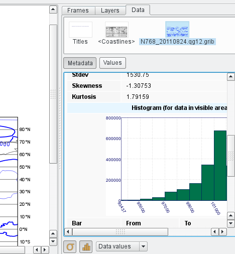
Histogram and statistics ON
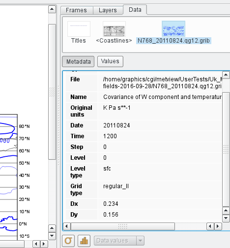
Histogram and statistics OFF
Avoid re-rendering
The least efficient way to plot a GRIB file is to perform the steps in this order:
visualise the file
drop a Contouring icon into the plot window
zoom into a smaller area
This will cause the data to be plotted a total of 3 times, 2 of which will be global.
A better strategy is this:
visualise a Geographic View icon that’s been set to the desired area (or global if desired)
drop the GRIB icon with a Contouring icon together into the plot window (plus any other icons required, e.g. Coastlines)
Now the data will be plotted just once, and only on the smaller area (if selected).
Choose your plotting algorithm wisely
For plotting larger areas (say, Europe or the whole globe), it can be best to switch to cell shading for a faster plot. For small areas (e.g. the size of a small country), grid shading will give the most accurate results, but this can be slower for larger areas.
Example grid shading parameters for LSM
MCONT,
   LEGEND     = ON,
   CONTOUR    = OFF,
   CONTOUR_MAX_LEVEL = 1.01,
   CONTOUR_SHADE_MAX_LEVEL = 1.01,
   CONTOUR_SHADE = ON,
   CONTOUR_SHADE_TECHNIQUE = CELL_SHADING,
   CONTOUR_SHADE_CELL_RESOLUTION = 50,
   CONTOUR_SHADE_MAX_LEVEL_COLOUR = KELLY_GREEN,
   CONTOUR_SHADE_MIN_LEVEL_COLOUR = 'RGB(0.95,0.97,0.98)',
   CONTOUR_SHADE_COLOUR_DIRECTION = CLOCKWISE
Download icon: cell_shade50
Example grid shading parameters for LSM
MCONT,
   LEGEND     = ON,
   CONTOUR    = OFF,
   CONTOUR_MIN_LEVEL = 0.0001,
   CONTOUR_SHADE_MIN_LEVEL = 0.0001,
   CONTOUR_SHADE = ON,
   CONTOUR_SHADE_TECHNIQUE = GRID_SHADING,
   CONTOUR_SHADE_MAX_LEVEL_COLOUR = KELLY_GREEN,
   CONTOUR_SHADE_MIN_LEVEL_COLOUR = 'RGB(0.95,0.97,0.98)',
   CONTOUR_SHADE_COLOUR_DIRECTION = CLOCKWISE
Download icon: grid_ shade
Keep an eye on memory usage
Run some kind of process monitor and sort by memory usage. Be ready to ‘kill’ the uPlot process if it’s taking too much memory!
Be careful when plotting to a file
The memory used during an on-screen interactive plot is released when the window is closed. But if you plot to a file (e.g. PNG, PDF, PS) the memory will not be released and you may have to kill the uPlotBatch process in order to release it.