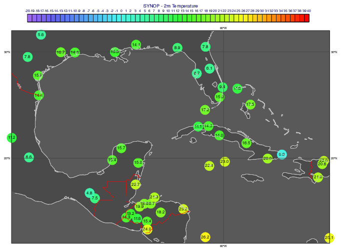
BUFR, Geopoints - Coloured Observation Values in Circles

# (C) Copyright 2017- ECMWF.
#
# This software is licensed under the terms of the Apache Licence Version 2.0
# which can be obtained at http://www.apache.org/licenses/LICENSE-2.0.
#
# In applying this licence, ECMWF does not waive the privileges and immunities
# granted to it by virtue of its status as an intergovernmental organisation
# nor does it submit to any jurisdiction.
#

import metview as mv

# read BUFR data
filename = "synop.bufr"
if mv.exist(filename):
    synop_bufr = mv.read(filename)
else:
    synop_bufr = mv.gallery.load_dataset(filename)

# filter just the 500 hPa temperature from the obs data (Geopoints)
gpt = mv.obsfilter(output="geopoints", parameter="airTemperatureAt2M", data=synop_bufr)

# convert values to C units
gpt = gpt - 273.16

# define coloured symbols (filled circles)
sym = mv.msymb(
    legend="on",
    symbol_type="marker",
    symbol_table_mode="advanced",
    symbol_advanced_table_selection_type="interval",
    symbol_advanced_table_interval=1,
    symbol_advanced_table_min_value=-20,
    symbol_advanced_table_max_value=40,
    symbol_advanced_table_max_level_colour="red",
    symbol_advanced_table_min_level_colour="lavender",
    symbol_advanced_table_colour_director="clockwise",
    symbol_advanced_table_marker_list=15,
    symbol_advanced_table_height_list=1.4,
)

# define value (as number) plotting
sym_text = mv.msymb(
    legend="off",
    symbol_table_mode="advanced",
    symbol_format="(F3.1)",
    symbol_advanced_table_selection_type="interval",
    symbol_advanced_table_interval=1000,
    symbol_advanced_table_max_level_colour="black",
    symbol_advanced_table_min_level_colour="black",
    symbol_advanced_table_colour_director="clockwise",
    symbol_advanced_table_text_display_mode="centre",
    symbol_advanced_table_text_font_size=0.35,
)

# shaded land and sea
coast = mv.mcoast(
    map_coastline_land_shade="on",
    map_coastline_land_shade_colour="RGB(0.29,0.29,0.29)",
    map_coastline_sea_shade="on",
    map_coastline_sea_shade_colour="RGB(0.35,0.35,0.35)",
    map_coastline_colour="RGB(0.79,0.79,0.79)",
    map_boundaries="on",
    map_boundaries_colour="red",
    map_grid_latitude_increment=10,
    map_grid_longitude_increment=20,
    map_grid_colour="RGB(0.25,0.25,0.25)",
)

# adjust the legend
legend = mv.mlegend(legend_text_font_size=0.3)

# define title
title = mv.mtext(text_lines="SYNOP - 2m Temperature", text_font_size=0.4)

# set the view area
view = mv.geoview(
    map_area_definition="corners", area=[12, -100, 32, -70], coastlines=coast
)

# define the output plot file
mv.setoutput(mv.pdf_output(output_name="coloured_obs_values_in_circles"))

# plot the data with the style
mv.plot(view, gpt, sym, sym_text, legend, title)