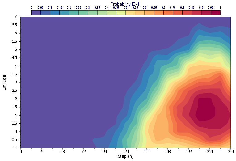
CSV - Gridded XY Data with Contouring

# (C) Copyright 2017- ECMWF.
#
# This software is licensed under the terms of the Apache Licence Version 2.0
# which can be obtained at http://www.apache.org/licenses/LICENSE-2.0.
#
# In applying this licence, ECMWF does not waive the privileges and immunities
# granted to it by virtue of its status as an intergovernmental organisation
# nor does it submit to any jurisdiction.
#

import metview as mv
import numpy as np
import pandas as pd
import xarray as xr

# This example demonstrates how to visualise gridded XY
# data stored in an ASCII format with contouring. Metview
# can only generate a plot like this for NetCDF data,
# so to achieve this goal we will convert the input data
# stored in a CSV file into NetCDF using pandas and xarray.

# get CSV file, contains probabilities per latitude band and timestep
# rows: latitudes, columns: forecast steps
filename = "matrix_prob.csv"
if not mv.exist(filename):
    mv.gallery.load_dataset(filename)

# read data into a pandas dataframe
df = pd.read_csv(filename, header=None)

# get data into a numpy array
v = df.to_numpy()

# the CSV file does not contain the X, Y coordinates, but we need
# to generate them
lats = [x for x in np.arange(7, -1.5, -0.5)]
steps = list(range(0, 252, 12))
# print(f"lats={lats}")
# print(f"steps={steps}")
# print(f"min={v.min()} max={v.max()}")

# create xarray dataset
ds = xr.Dataset(
    data_vars=dict(
        prob=(["lat", "step"], v),
    ),
    coords=dict(
        lat=(["lat"], lats),
        step=(["step"], steps),
    ),
    attrs=dict(description="Probability"),
)
# save xarray to netcdf and read it back a Metview object
tmp_nc_filename = "_xy_tmp.nc"
ds.to_netcdf(tmp_nc_filename)
f = mv.read(tmp_nc_filename)

# define visualiser
vis = mv.netcdf_visualiser(
    netcdf_data=f,
    netcdf_plot_type="xy_matrix",
    netcdf_x_variable="step",
    netcdf_y_variable="lat",
    netcdf_value_variable="prob",
)

# Define horizontal axis
hor_axis = mv.maxis(
    axis_orientation="horizontal",
    axis_title_text="Step (h)",
    axis_title_height=0.6,
    axis_tick_interval=24,
    axis_tick_label_height=0.5,
    axis_minor_tick="on",
    axis_minor_tick_count=1,
    axis_grid="on",
    axis_grid_colour="black",
    axis_grid_line_style="dot",
)

# Define vertical  axis
ver_axis = mv.maxis(
    axis_position="left",
    axis_title_text="Latitude",
    axis_title_height=0.6,
    axis_tick_interval=0.5,
    axis_tick_label_height=0.5,
    axis_minor_tick="on",
    axis_minor_tick_count=2,
    axis_grid="on",
    axis_grid_colour="black",
    axis_grid_line_style="dot",
)

# Define Cartesian view
view = mv.cartesianview(
    # x_min=-1,
    # x_max=1,
    y_min=-1,
    y_max=7,
    x_automatic="on",
    y_automatic="off",
    subpage_y_position=12.5,
    subpage_y_length=75,
    horizontal_axis=hor_axis,
    vertical_axis=ver_axis,
)

# define contour shading
cont_shade = mv.mcont(
    legend="on",
    contour="off",
    contour_level_selection_type="interval",
    contour_shade_max_level=1,
    contour_shade_min_level=0,
    contour_interval=0.05,
    contour_label="off",
    contour_shade="on",
    contour_shade_colour_method="palette",
    contour_shade_method="area_fill",
    contour_shade_palette_name="colorbrewer_Spectral_14",
)

title = mv.mtext(
    text_lines=["Probability [0-1]"],
    text_font_size=0.6,
)

# define legend
legend = mv.mlegend(legend_text_font_size=0.4)


# define the output plot file
mv.setoutput(mv.pdf_output(output_name="xy_gridded_ascii"))

# generate plot
mv.plot(view, vis, cont_shade, title, legend)