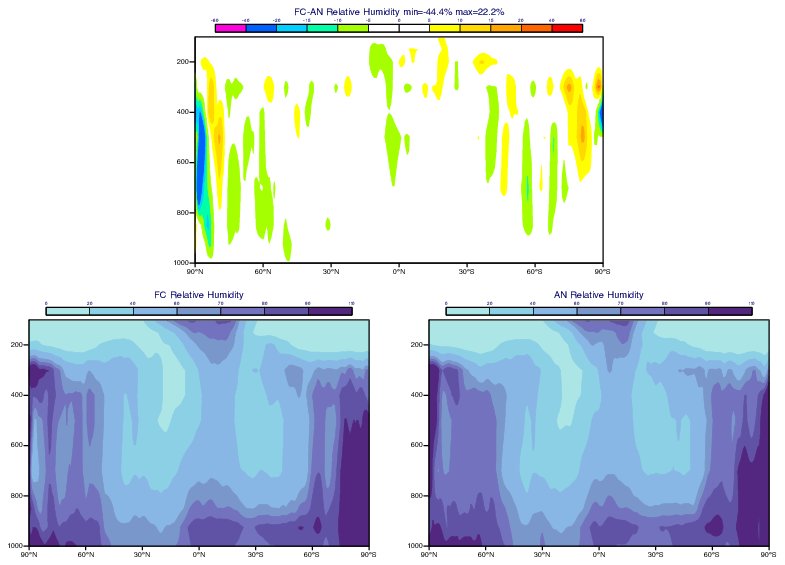
GRIB - Zonal Average Difference

# (C) Copyright 2017- ECMWF.
#
# This software is licensed under the terms of the Apache Licence Version 2.0
# which can be obtained at http://www.apache.org/licenses/LICENSE-2.0.
#
# In applying this licence, ECMWF does not waive the privileges and immunities
# granted to it by virtue of its status as an intergovernmental organisation
# nor does it submit to any jurisdiction.

import numpy as np
import metview as mv

# getting data
use_mars = False

# getting forecast data from MARS
if use_mars:
    ret_core = {
        "param": "r",
        "time": 0,
        "levtype": "pl",
        "levelist": [1000, 925, 850, 700, 500, 400, 300, 200, 150, 100],
        "grid": [1, 1],
    }
    an = mv.retrieve(type="an", date=20210226, **ret_core)
    fc = mv.retrieve(type="fc", date=20210221, step=120, **ret_core)

# read data from file
else:
    filename = "r_an_global_upper.grib"
    if mv.exist(filename):
        an = mv.read(filename)
    else:
        an = mv.gallery.load_dataset(filename)

    filename = "r_fc_global_upper.grib"
    if mv.exist(filename):
        fc = mv.read(filename)
    else:
        fc = mv.gallery.load_dataset(filename)

# define the "zonal" average view
view = mv.maverageview(bottom_level=1000, top_level=100, direction="ew")

# define the layout
page_0 = mv.plot_page(bottom=50, left=20, right=80, view=view)

page_1 = mv.plot_page(top=50, bottom=100, right=50, view=view)

page_2 = mv.plot_page(top=50, left=50, view=view)

dw = mv.plot_superpage(pages=[page_0, page_1, page_2])

# define contour shading for r
cont = mv.mcont(
    legend="on",
    contour="off",
    contour_level_selection_type="level_list",
    contour_level_list=[0, 20, 40, 60, 70, 80, 90, 110],
    contour_label="off",
    contour_shade="on",
    contour_shade_colour_method="palette",
    contour_shade_method="area_fill",
    contour_shade_palette_name="eccharts_blue_purple_7",
)

# define contour shading for differences
diff_cont = mv.mcont(
    legend="on",
    contour="off",
    contour_level_selection_type="level_list",
    contour_max_level=60,
    contour_min_level=-60,
    contour_level_list=[-60, -40, -20, -15, -10, -5, 0, 5, 10, 15, 20, 40, 60],
    contour_label="off",
    contour_shade="on",
    contour_shade_colour_method="palette",
    contour_shade_method="area_fill",
    contour_shade_palette_name="eccharts_blue_red_12",
)

# generate the zonal mean of the forecast
d_fc = mv.mxs_average(data=fc, direction="ew")

# generate the zonal mean of the analysis
d_an = mv.mxs_average(data=an, direction="ew")

# generate the zonal mean of the difference
d_diff = mv.mxs_average(data=fc - an, direction="ew")

# compute the min an max of the zonal mean of the difference. The
# zonal mean data is a NetCDF object. The variable holding the data in
# this case is called "r" (this is the ecCodes shortName in the input GRIBs)
mv.setcurrent(d_diff, "r")
min_v = np.amin(mv.values(d_diff))
max_v = np.amax(mv.values(d_diff))

# define difference title
title_diff = mv.mtext(
    text_lines="FC-AN Relative Humidity min={:.1f}% max={:.1f}%".format(min_v, max_v),
    text_font_size=0.4,
)

# define other titles
title_fc = mv.mtext(text_lines="FC Relative Humidity", text_font_size=0.4)
title_an = mv.mtext(text_lines="AN Relative Humidity", text_font_size=0.4)

# define the output plot file
mv.setoutput(mv.pdf_output(output_name="zonal_average_difference"))

# generate plot
mv.plot(
    dw[0],
    d_diff,
    diff_cont,
    title_diff,
    dw[1],
    d_fc,
    cont,
    title_fc,
    dw[2],
    d_an,
    cont,
    title_an,
)