VAPOR Tutorial
This tutorial explains how to convert ECMWF GRIB data into VAPOR format and how to visualise the resulting data in VAPOR.
Note
Please note that this tutorial requires Metview version 4.4.6 or later. Also for users outside ECMWF the Metview VAPOR interface should be properly set up as described :ref:`here <vapor_setup>`_.
Preparations
First start Metview; at ECMWF, the command to use is metview (see Metview at ECMWF for details of Metview versions). You should see the main Metview desktop popping up.
You will create some icons yourself, but some are supplied for you - please download the following file:
Alternatively, if at ECMWF then you can copy it like this from the command line:
cp /home/graphics/cgx/tutorials/vapor_tutorial.tar.gz $HOME/metview
and save it in your $HOME/metview directory. You should see it appear on your main Metview desktop, from where you can right-click on it, then choose execute to extract the files.
You should now (after a few seconds) see a vapor_tutorial folder which contains the solutions and also some additional icons required by these exercises.
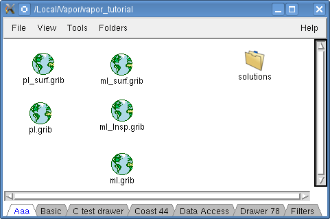
You will work in the vapor_tutorial folder so open it up. You should see the following contents:
VAPOR Basics
VAPOR stands for Visualization and Analysis Platform for Ocean, Atmosphere, and Solar Researchers. It is a software system providing an interactive 3D visualization environment. The home of the software is https://www.vapor.ucar.edu.
VAPOR input files
VAPOR input data is described by .vdf (VAPOR Data Format) files. These are XML files containing the name and dimension of all the variables and the path of the actual data files storing the data values. VAPOR stores its data values in .vdc (VAPOR Data Collection) files. These are NetCDF files containing wavelet compressed 3D data. There is a separate file for each variable and timestep organized into a folder hierarchy.
There are a set of VAPOR command line tools that can convert NetCDF input data into this format but there is no such tool available for GRIB. This tutorial shows you how to use Metview’s VAPOR Prepare icon icon to convert GRIB data into the VAPOR format.
VAPOR grids
VAPOR input data must be defined on a 3D grid, which has to be regular horizontally (on a map projection).
It is crucially important to understand the vertical coordinate types of the input data VAPOR can use. Here we discuss only the two types that the Metview VAPOR interface supports
For layered grids VAPOR expects a parameter specifying the elevation of each 3D level in the input data. This is typically the case for pressure or model level (n levels) data with height or geopotential available (or it can be computed).
For regular grids the 3D levels are supposed to be equidistant (in the user coordinate space). This type can be used when the data is available on equidistant height levels.
When pressure or model level data is present without height information the situation is somewhat special. The grid in this case is not layered but can be regarded as regular in its own coordinate space (pressure or model levels) letting the z axis simply represent pressure or model levels in the 3D scene rendered in VAPOR.
VAPOR uses a right-handed coordinate system which means that :
the horizontal grid has to start at the SW corner
the vertical coordinates have to increase along the z axis (upwards)
Supported GRIBs
Only GRIB fields on a regular lat-lon grid are supported at the moment. However, please note that GRIBs can be internally interpolated to a regular lat-lon grid by using the VAPOR_AREA_SELECTION parameter. The parameters to be converted are supposed to have the same validity date and time and the same vertical levels. They also have to be valid on the same grid.
Converting pressure level data with elevation
This exercise demonstrate how to use pressure level ECMWF GRIB data with VAPOR when elevation (as geopotential) is available. We will work with fields on a low resolution grid over Europe.
Getting the GRIB data
The GRIB data is already in its place. In your folder you will find the two GRIB files you need to use for this exercise:
pl.grib: contains z, t, r, u and v on pressure levels
pl_surf.grib: contains z, 2t ,10u and 10v on surface
Please note that both these files were retrieved from MARS by using the ‘ret_pl’ and ‘ret_pl_surf’ MARS retrieval icons in the solutions folder.
Running Vapor Prepare
Create a VAPOR Prepare icon icon (right-click in the desktop when no icons are selected and use the New icon … menu).

Rename it ‘vapor_pl’ and open up its editor.
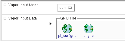
First, ensure that Vapor Input Mode is set to ‘Icon’ then drop the two Mars Retrieval icons into the Vapor Input Data field.
Then you need to define the list of GRIB parameters you want to see in VAPOR.
Vapor 2d Params |
z/2t/10u/10v |
Vapor 3d Params |
t/u/v/r |
Note
Internally VAPOR Prepare icon converts surface geopotential to metres and rename it HGT.
The vertical coordinate system has to be set carefully:
Vapor Vertical Grid Type |
Layered |
Vapor Elevation Param |
z |
Vapor Bottom Coordinate |
0 |
Vapor Top Coordinate |
16000 |
Here you set the vertical grid type to ‘Layered’ and defined geopotential (z) as the parameter holding the elevation of the vertical layers (pressure levels). You also specified the vertical coordinate range (in metres) that VAPOR will display.
Note
Internally VAPOR Prepare icon converts geopotential to metres and rename it ELEVATION (this is required by VAPOR).
The last step is to specify the name and location of the results of the conversion:
Vapor Vdf Name |
tut_pl |
Vapor Output Path |
your_path_on_the_filesystem |
With these settings a VDF file called ‘tut_pl.vdf’ will be created in the directory you specified. All the other VAPOR data files will be placed into a subdirectory called ‘tut_pl_data’.
Note
This tutorial works only with a small amount of data. However, real life examples can easily result in huge VAPOR files (gigabytes). Therefore you should always carefully select the output path for the GRIB to VAPOR conversion.
Now save your VAPOR Prepare icon icon then right click Execute to run the conversion. The icon will first turn orange then green when the conversion finishes.
To visualise the VAPOR data generated please follow the instructions here.
Converting model level data with elevation
This exercise demonstrate how to use model level ECMWF GRIB data with VAPOR when elevation available/can be derived. We will work with fields on the same low resolution grid over Europe as we used for the pressure levels.
Getting the GRIB data
The GRIB data is already in its place. In your folder you will find the three GRIB files you need for this exercise:
ml.grib: contains q, t, u and v on model levels 137-60
ml_lnsp.grib: contains lnsp on the bottommost model level (level 137)
ml_surf.grib: contains z, 2t ,10u and 10v on surface).
Please note that these files were retrieved from MARS by using the ‘ret_ml’, ‘ret_ml_lnsp’ and ‘ret_ml_surf’ MARS retrieval icons in the solutions folder.
Note
Please note that upper level geopotential (z) is not available in the input files because it is not archived in MARS for model levels. However, VAPOR Prepare icon can derive it if tempreature (t), specific humidity (q) and logarithm of surface pressure (lnsp) are available (it is the case for our input data).
Running Vapor Prepare
Create a VAPOR Prepare icon icon. Rename it ‘vapor_ml’ and open up its editor.
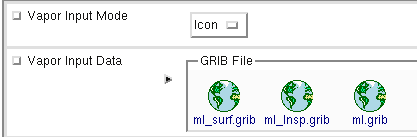
First, ensure that Vapor Input Mode is set to Icon then drop your three Mars Retrieval icons into the Vapor Input Data field.
Then you need to define the list of GRIB parameters you want to see in VAPOR.
Vapor 2d Params |
z/2t/10u/10v |
Vapor 3d Params |
t/u/v/q |
The vertical coordinate system has to be set carefully:
Vapor Vertical Grid Type |
Layered |
Vapor Elevation Param |
z |
Vapor Bottom Coordinate |
0 |
Vapor Top Coordinate |
16000 |
Here you set the vertical grid type to layered and defined geopotential (z) as the parameter holding the elevation of the vertical layers (model levels). We also specified the vertical coordinate range (in metres) that VAPOR will display for this data.
Note
Although geopotential (z) is not available on model levels in the input data VAPOR Prepare icon computes it automatically if tempreature (t), specific humidity (q) and logarithm of surface pressure (lnsp) are available. Geopotential then gets converted into metres units and renamed to ELEVATION.
Last, we specify the name and location of the results of the conversion:
Now save your VAPOR Prepare icon icon then right click Execute to run the conversion. The icon will first turn orange then green when the conversion finishes.
To visualise the VAPOR data generated please follow the instructions in the next chapter.
Visualisation
Note
Giving detailed instructions about VAPOR visualisation goes beyond the scope of this tutorial. Here you will learn only the basics about how to visualise 3D data with VAPOR. F or an in depth introduction please study the VAPOR tutorials at:
Stating up VAPOR
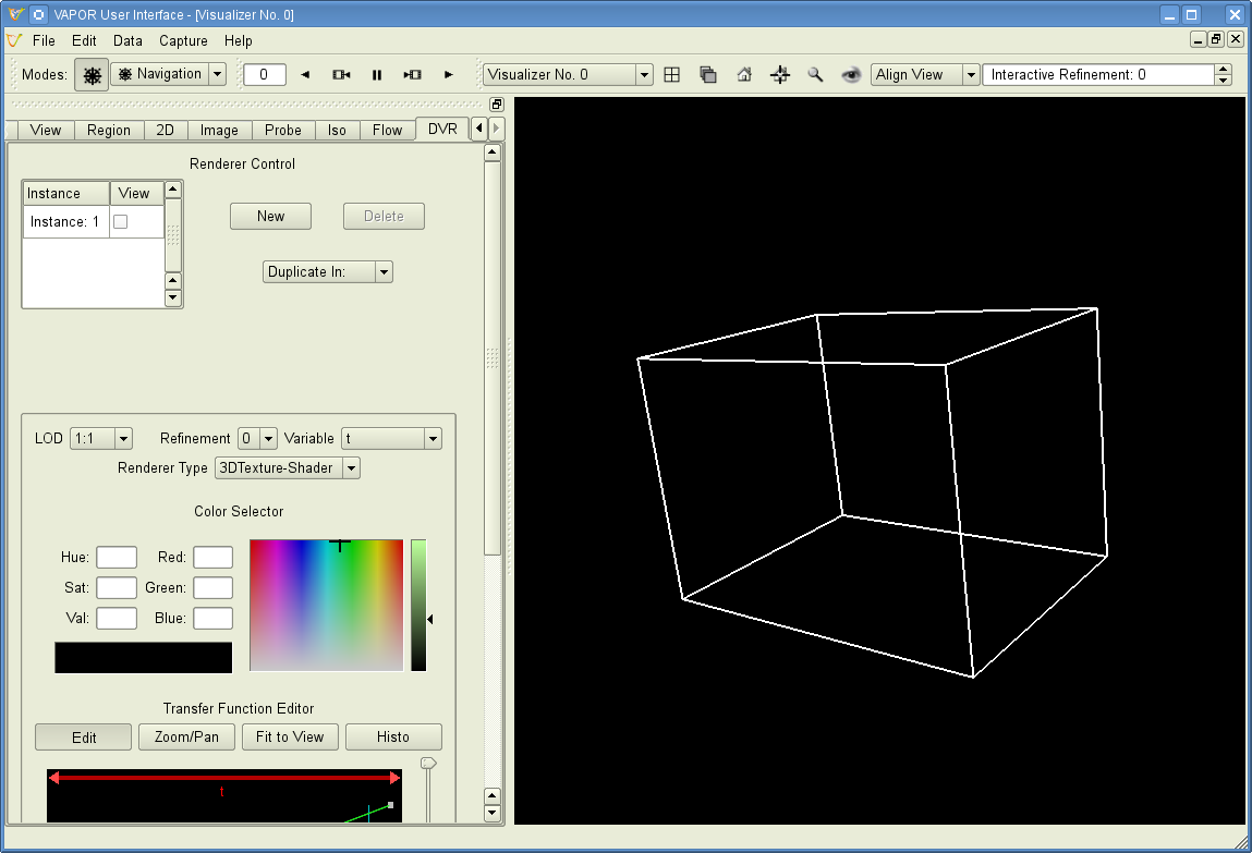
Right click Visualise your VAPOR Prepare icon icon to start up VAPOR. You will see this window popping up:
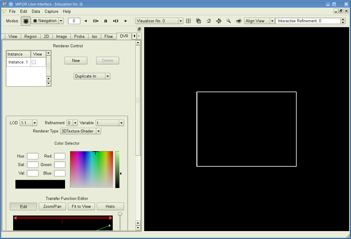
Your vdf file (that you have created with your VAPOR Prepare icon icon) is now loaded into VAPOR and you can see a cube representing your 3D data volume.
Adjusting the view volume
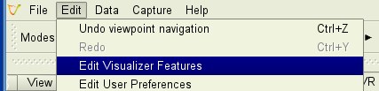
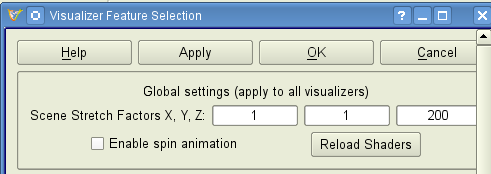
If you rotate the cube in the display window (left mouse button) you will see it is flat. We need to scale the vertical axis to get a better view of the whole 3D volume. Go to the Edit -> Edit Visualiser Features menu and set the Z Scene Stretch Factor to 200:
Now the full 3D volume is visible:
Setting up the map image
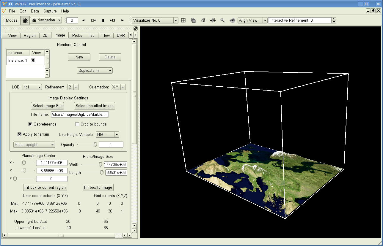
We can load a pre-installed map image to get a better geographical reference for the domain we are looking at. Open the Image tab and load ‘BigBlueMarble.tiff’ by using the Select Installed Image button. Then tick Instance: 1, tick Apply to Terrain and set Z to 0. The scene has now changed like this:
The VAPOR session file
The current scene settings can be saved into a VAPOR session file (with a .vss suffix) by using the File -> Save Session (As) menu. Then next time we start up VAPOR the saved session files can be loaded to initialise the scene with the saved settings.
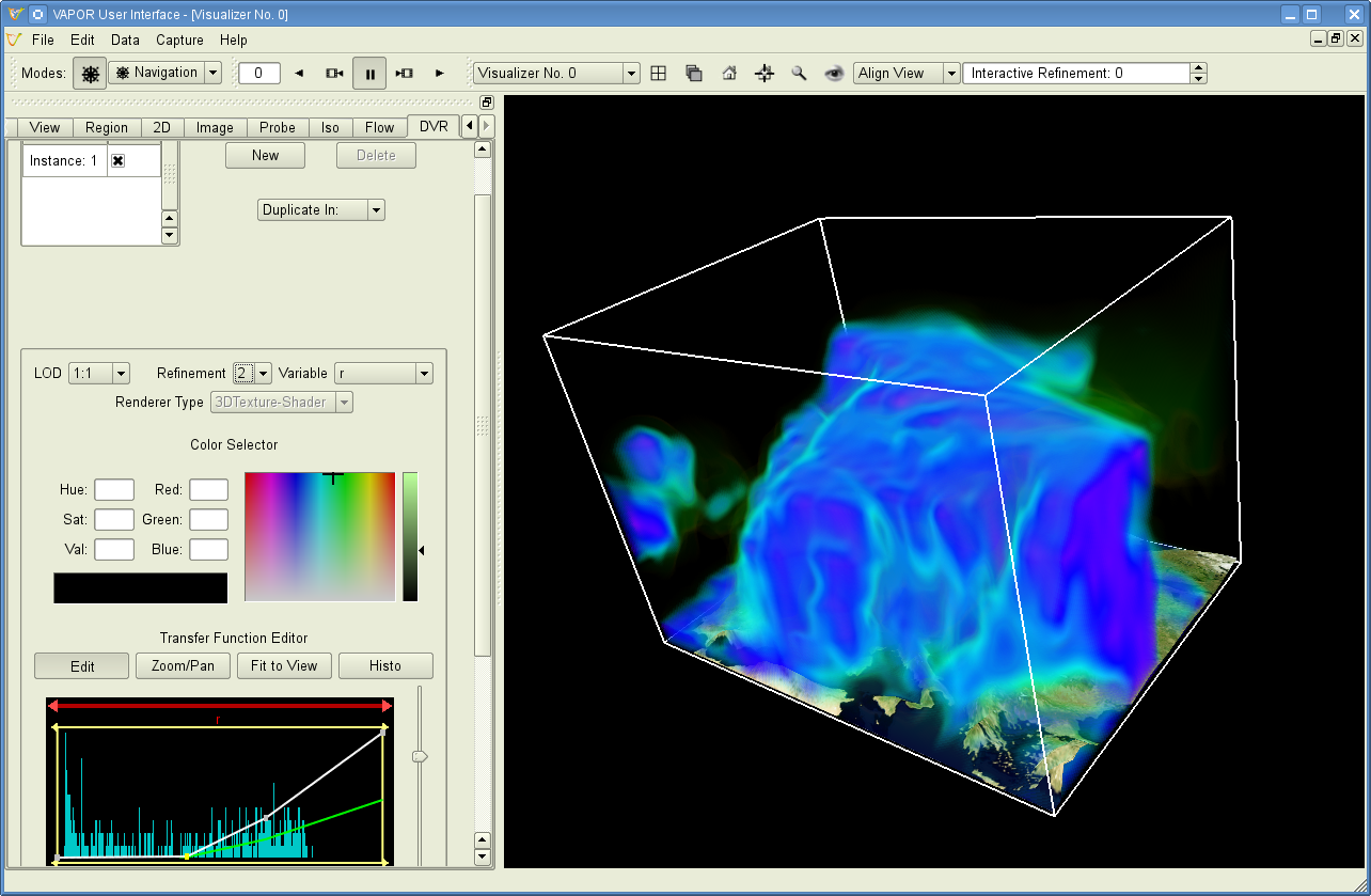
Direct volume rendering (DVR)
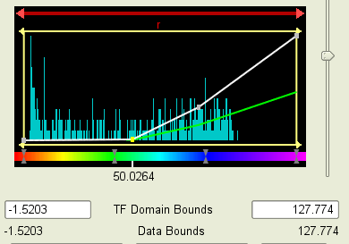
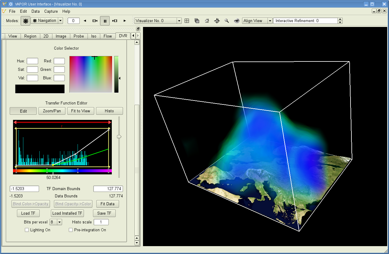
Having set up the view you can now visualise our data. Click on the DVR (Direct Volume Rendering) tab, select Variable to relative humidity (r), tick Instance 1. Then change the opacity in the Transfer Function editor like this (drag the control points of the white curve and use the vertical slide on the right of the histogram):
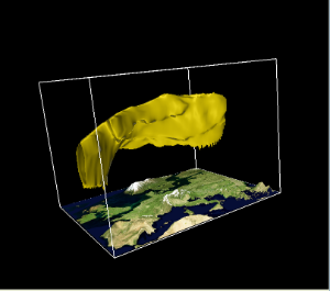
Having done so you should get this scene:
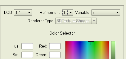
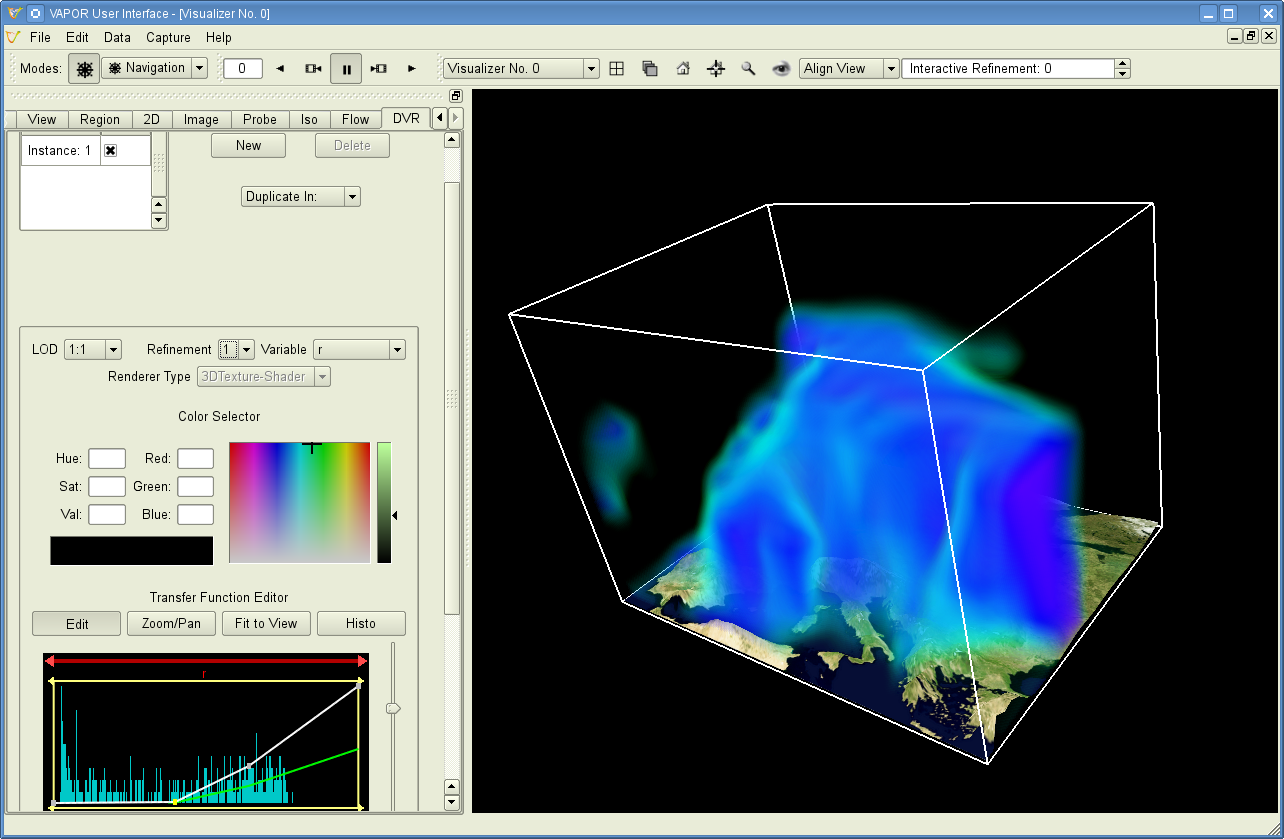
Please note that this scene was generated by using only low resolution data. The see more details change the Refinement level first to 1 then to 2.
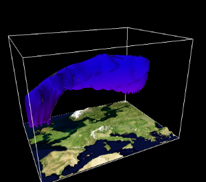
You should see more details appear in the scene:
Further rendering types
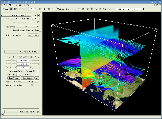
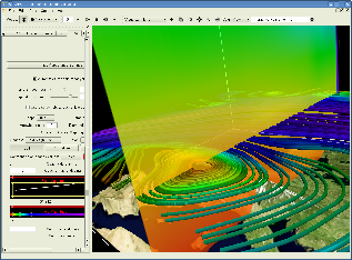
There are other types of renderers which we just list here and present a small gallery made with the data used for this tutorial:
wind barb plotting: see the Barbs tab
2D field plotting: see the 2D tab
cross sections: see the Probe tab
flow visualisation (streamlines): see the Flow tab
iso surfaces: see the Iso tab
Note
For further details please study the VAPOR tutorials at: