ODB Tutorial 2
Note
Please note that this tutorial was designed to be used only at ECMWF.
Preparations
First start Metview; at ECMWF, the command to use is metview for this tutorial (see Metview at ECMWF for details of Metview versions).
Then run the following command from the command line:
cp -Rf ~cgx/tutorials/odb_seminar_2017 ~/metview/
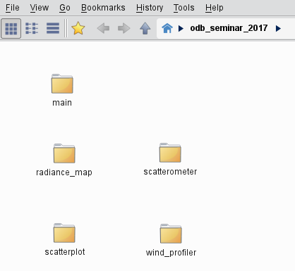
This will copy all the examples into your Metview home folder. Soon you will see a folder called ‘odb_seminar_2017’ appear on your main Metview desktop. Double-click to enter it. You should see the following contents:
ODB Exercise
This exercise shows how to retrieve ODB data from MARS, examine its structure then plot and process it in different ways. Enter folder ‘main’ to start the exercise.
Retrieving the ODB data from MARS
The ‘ret_temp’ MARS Retrieval icon is already prepared for you to fetch Land TEMP ODB data from MARS for a given date. Edit the icon (right-click & edit) to see what parameters are set. The most important ones are as follows:
Parameter |
Value |
Notes |
Type |
MFB |
Mondb feedback |
Obsgroup |
17 |
Conventional |
Reportype |
16022 |
land TEMP |
Close the icon editor and perform the data retrieval by choosing execute from the icon’s context menu. The icon name should turn orange whilst the retrieval takes place, then green to indicate success.
Note
If ‘ret_temp’ does not turn green after half a minute probably there is a problem with MARS. In this case find the the ‘backup.temp.odb’ ODB Database icon at the top-right of the folder and rename it ‘temp.odb’ (right-click and rename). This icon contains the very same data that we wanted to retrieve from MARS.
If the MARS retrieval was successful the data is now cached locally. To see what was retrieved, right-click examine the icon. This brings up Metview’s ODB Examiner tool. Here you can see the metadata (Columns tab) and the actual data values themselves as well (Data tab). Close the ODB Examiner.
To save the ODB data from the cache to disk, right-click Save result on the Mars Retrieval icon and save as ‘temp.odb’. A few seconds later an ODB Database icon with the given name will appear at the bottom of your folder.
Using the ODB Visualiser
We will visualise the 500 hPa temperature values from our ODB using the ‘vis_temp’ ODB Visualiser icon. The query we need to perform is as follows:
select
  lat@hdr,
  lon@hd,
  obsvalue@body
where
  varno = 2 and vertco_reference_1=50000
Now edit the ‘vis_temp’ icon.
First, drop your ODB Database icon into the ODB Data field.
Next, specify the where statement of the query in the ODB Where parameter as:
varno = 2 and vertco_reference_1=50000
Save these settings by clicking the Save button at the bottom-right of the icon editor (or click Ok to save and close the editor).
Right-click visualise the ‘vis_temp’ icon to generate the plot. Then drag the the provided Symbol Plotting, Coastlines, Legend and Text Plotting icons into the plot for further customisation. Keep the plot window open.
Inspecting the Data Values in the Plot
Data values at the cursor position can be inspected with the Cursor Data Tool, which can be activated by pressing on the

icon in the toolbar of the Display Window. The Cursor Data Tool displays the co-ordinates of the current cursor position and the information for the nearest data point to this position.
You may find it hard to use the Cursor Data Tool in data dense regions. To overcome this launch the Magnifier with the

icon in the toolbar and move it to your area of interest in the plot. The magnifying glass can be moved and resized using the mouse, and the magnification scale on its left-hand side can also be adjusted. You can also zoom into areas of the map using the Zoom controls
in the toolbar.
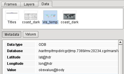
Enable the sidebar of the Display Window with the

button and select the Data tab (and select the ‘vis_temp’ layer at the top if it is not yet selected). Now select the Metadata panel inside the tab. Here you will find some statistics about the data plotted and a histogram as well.
Now switch to the Values panel. This features a list showing all the plotted data. In the bottom-left corner click on the

button to activate the Data probe (this will appear in the plot). The probe is synchronised with the list. Try to drag it around in the plot, or change its position through the list. The Magnifier might help you position the Data probe more accurately.
Writing a Macro
We will write a Macro to reproduce the same temperature map as we plotted with icons.
Create a new Macro icon (in an empty area of the desktop right-click and select Create new macro) and edit it. First, drag your ‘vis_temp’ ODB Visualiser icon into the Macro editor just below the line containing the #Metview Macro text.
Next, drag your ‘symbol’ Symbol Plotting icon into the editor below the text the editor already holds. Next, add the following line to the macro:
plot(vis_temp,symbol)
Now click on the play button

in the Macro editor to run the Macro. You should see a nice plot popping up.
A more advanced version of this macro is provided for you as ‘plot_map.mv’. It features all the icons we used to customise the original plot, allows selection of the pressure level to plot and automatically adjusts the symbol plotting to current value range.
Overlaying with GRIB data
The ‘fc.grib’ GRIB icon contains a 12 h global forecast valid for the date and time of our TEMP ODB data. Double-click the icon to inspect its fields with the GRIB Examiner.
Re-visualise the 500 hPa temperature ODB data with vis_temp’ and drag the Symbol Plotting, Coastlines, Legend and Text Plotting icons into the plot again. To overlay the 500 hPa temperature forecast we need to filter the matching field from the GRIB file. The ‘t500_fc’ GRIB Filter icon is already already set up to perform this task. Just drag it into the plot, then drag the ‘t_cont’ Contouring icon into the plot as well to customise the contour lines.
Forecast-observation difference
The ‘diff.mv’ Macro computes the difference between the forecasts stored in the ‘fc.grib’ GRIB file and the observations stored in the ‘temp.odb’ ODB. This is achieved by using the following steps:
the ODB query is performed and the resulting data is converted into Geopoints (this is Metview’s own format to store scattered geospatial data)
the matching GRIB field is read and interpolated to the observation points
the difference is computed between forecast and observation
Edit ‘diff.mv’ and visualise it using the play button. Try to set a different level/parameter by changing parameters lev and odb_par at the top of the macro code.
Wind plotting
The ‘plot_wind.mv’ Macro plots wind on a given pressure level from the ‘temp.odb’ ODB. It is not a trivial task to do because the u and v wind components cannot be retrieved from our ODB with a single query. This macro overcomes this difficulty by using the following steps:
two ODB queries are performed: one for the u and one for the v wind component
the resulting data is converted into Geopoints
the wind data plotted as Geopoints
Edit ‘plot_wind.mv’ and visualise it using the play button.
Try to set a different level by changing parameter lev at the top of the macro code.
Tephigram plotting
Macro ‘plot_tephi.mv’ demonstrates how to extract and plot TEMP ODB data into a tephigram (it is a type of thermodynamic diagram for atmospheric profiles). Edit the macro and visualise it. Try to change the station specified at the top of the macro code.
Other Examples
There are some other examples provided in ‘odb_seminar_2017’ folder (it is one level up from folder ‘main’).
Satellite radiances
Enter folder ‘radiance_map’.”ASMUA.odb” stores AMSU-A brightness temperature observations. Use ‘tb_plot’ to visualise it and the other provided icons to customise the plot.
Scatterometer wind
Enter folder ‘scatterometer’.
‘SCATT.odb’ contains scatterometer data. Macro ‘scatt.mv’ extracts and plots scatterometer wind (ambiguous wind components) for a limited area and time period. Visualise the macro and drop the provided ‘mslp.grib’ icon into the plot. This GRIB contains a mean sea level forecast valid at the same time as the observations.
Scatterplot
Enter folder ‘scatterplot’.
“ASMUA.odb” stores AMSU-A brightness temperature observations.
Visualise ‘scatter_plot’ and customise it with the provided Symbol Plotting icon. The plot you see is a scatterplot for the first guess departures (x axis) and analysis departures (y axis) for a given channel.
Visualise ‘bin_plot’ to get the binned version of the same data (as a heat map). Drop the provided Contouring, Cartesian View and Text Plotting icons into the plot to fully customise it.
Wind profiler
Enter folder ‘wind_profiler’.
‘PROF.odb’ contains wind profiler data. Use ‘profiler.mv’ to plot this data into a time-height diagram for a selected station.