plot_xs

plot_xs(*args, line=None, map_data=None, map_line=True, view=None, area=None, title_font_size=0.4, legend_font_size=0.35)

New in metview-python version 1.8.0

High level function with automatic styling to generate cross section plots with a fixed layout.

Parameters

line (list) – specifies the cross section transect line as [lat1, lon1, lat2, lon2].
map_data (Fieldset or tuple/list of Fieldset and visual definition objects) – specifies the GRIB data (and the corresponding styles) that will be displayed in the side map. If map_data is None and map_line is False no side-map is displayed.
map_line (bool) – controls wether the cross section line is rendered onto the side map. The line style is hard-coded (thick red line).
view (geoview()) – specifies the map view as a geoview() for the side map. If area is also specified the projection in the view is changed to cylindrical (but the map style is kept). See make_geoview() on how to build a view with predefined areas and map styles.
area (str or list) – specifies the map area for the side map. It can be either a named built-in area or a list in the format of [S, W, N, E]. When area is a list a cylindrical map projection is used.
title_font_size (number) – specifies the font size in cm for the plot title
legend_font_size (number) – specifies the font size in cm for the plot legend

plot_xs() is a convenience function allowing to plot data in a simple way using predefined settings. The layout is always fixed containing two views: an optional side map and the cross section itself.

Side map

The side-map can display user specified GRIB data and the cross section line. See map_data and map_line.

Cross section

The data and the styles used to generate the cross section are defined by the positional arguments (*args). In the argument list a Fieldset can be followed by any number of visual definitions (mcont() and mwind()), which define the plotting style for the given data. If no style is specified for a data object the style will be automatically generated using the currently loaded style configuration.

Limitations

plot_xs() is a high-level function using pre-defined settings, therefore it comes with certain limitations:

each Fieldset must be defined on pressure levels and can only contain a single time instance (same sate, time step etc.)

the cross section view properties (e.g. level range, axes etc.) cannot be controlled

while the data and map view styles can be fully customised, the title and legend are automatically built and no control is offered over them

Note

If you would like to create a fully customised cross section plot see the cross section gallery examples.

Examples

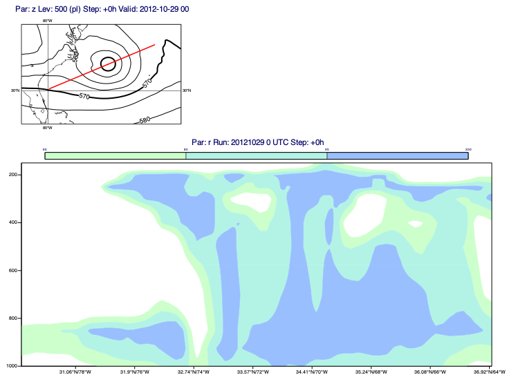
The following example shows how to create a cross section with relative humidity with a side map showing geopotential on 500 hPa:

import metview as mv

mv.setoutput("jupyter")

filename = "sandy_pl_025.grib"
if mv.exist(filename):
    g = mv.read(filename)
else:
    g = mv.gallery.load_dataset(filename)

r = g["r"]
z = g["z500"]

line = [30.30, -79.83, 36.95, -63.92]
mv.plot_xs(r, line=line, map_data=z, area=[25, -84, 40, -60], title_font_size=0.5)

Notebooks using `metview.plot_xs`

Working with datasets