Dataset plotting styles

Note

The Working with datasets notebook gives an overview of how to work with a dataset.

Using plot_maps()

Fields from a dataset can be plotted with plot_maps(), which is using a predefined style (when available) for each parameter.

The following code:

import metview as mv
ds = mv.load_dataset("demo")

run = mv.date("2016-09-25 00:00")
step = [0, 24, 48, 72, 96]

op = ds["oper"].select(date=run.date(), time=run.time(), step=step)
msl = op["msl"]
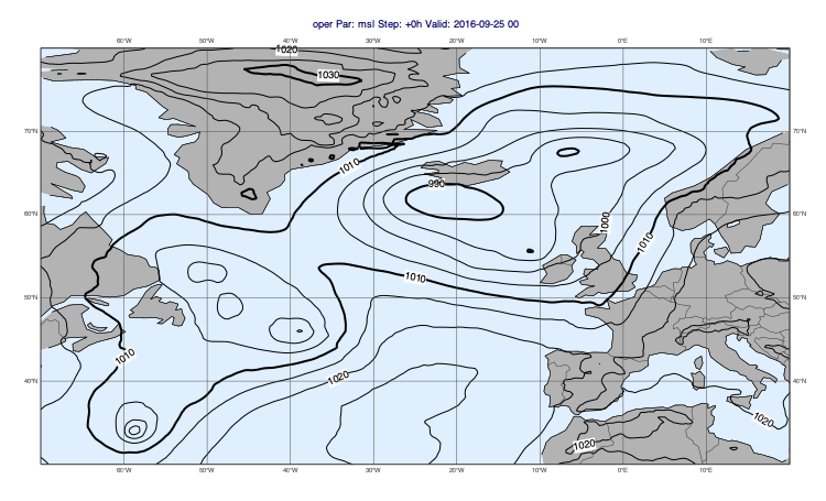
mv.plot_maps(msl)

generates the following plot with the default style assigned to the mean sea level pressure (“msl”):

Using a custom style

We can define our own mcont() to define a custom style:

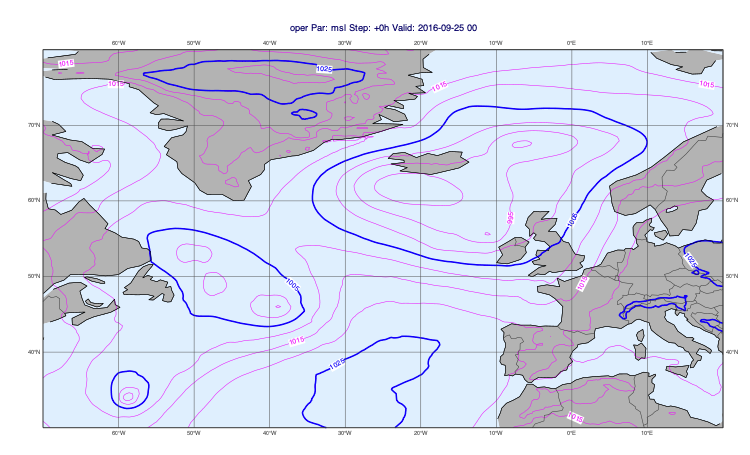
vd = mv.mcont({"contour_line_colour": "purple"})
mv.plot_maps(msl, vd)

Updating the default style

We can use ds_style() the get the associated default style for a given fieldset:

s = msl.ds_style()
print(s)

Style[name=msl] Visdef[verb=mcont, params={'legend': 'off',
 'contour_highlight_colour': 'black',
 'contour_highlight_thickness': 4, 'contour_interval': 5, 'contour_label': 'on',
 'contour_label_frequency': 2, 'contour_label_height': 0.4,
 'contour_level_selection_type': 'interval', 'contour_line_colour': 'black',
 'contour_line_thickness': 2, 'contour_reference_level': 1010}]

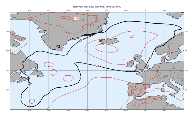
We can create a new style out of it with update() and pass it to plot_maps():

s1 = s.update({"contour_interval": 10, "contour_line_colour": "red"})
mv.plot_maps(msl, s1)

Getting the available styles

We can print the list of available styles for a fieldset:

print(msl.ds_style_list())

['msl', 'default_mcont']

Then we can get a style object by name:

s = mv.style.find('default_mcont')
print(s)

Style[name=default_mcont] Visdef[verb=mcont, params={'contour_automatic_setting': 'ecmwf', 'legend': 'on'}]

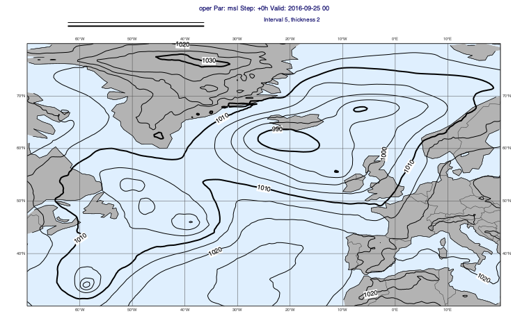
and pass it to plot_maps():

mv.plot_maps(msl, s)

Altering the style with update works in the same way as was shown for the default style above.