Track object
- class Track(path, skiprows=0, sep=' ', date_index=0, time_index=1, lat_index=2, lon_index=3)
Object to represent a geographical track (e.g. storm track) defined in a CSV file.
- Parameters
path (str) – specifies the CSV file containing the track data
skiprows (number) – skips the given number of rows from the CSV file (must be equal to the number of header rows at the beginning of the file)
sep (str) – the field separator character in the CSV data. When
sepis ” ” (a single whitespace) multiple whitespace separators are allowed in the CSV file.date_index – the index of the date column in the CSV file
time_index – the index of the time column in the CSV file
lat_index – the index of the latitude column in the CSV file
lon_index – the index of the longitude column in the CSV file
Trackallows for loading and plotting CSV track data in a simplified way. It can be used withplot_maps()to generate plots with pre-defined track styles.
How to use a Track?
The following CSV file is taken from the Storm track gallery example and has the following structure:
20121027 00 -76.9 27.1
20121027 12 -76.29 28.37
20121028 00 -74.64  30.2
20121028 12 -73.07 31.77
20121029 00 -70.87 33.66
...
So this data contains no header and the separator is a whitespace. Using
Trackwe can make plot in a few lines:import metview as mv filename = "sandy_track.grib" if mv.exist(filename): g = mv.read(filename) else: g = mv.gallery.load_dataset(filename) tr = mv.Track(path, sep=" ") mv.plot_maps(tr, view=mv.make_geoview(style="grey_2", area="north_america"))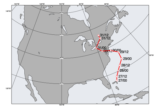
Compare this code to the one used in the gallery example to see how much we can simplify the plotting with
Track.
Customising the style
The style for
Trackis taken from the current style configuration. The default style is a list of anmgraph()(defining the curve) and anmsymb()(defining the labels), in that order. The main difficulty is that the labels must be added as a list of str to themsymb(), therefore the style is not fixed but must always be generated from the current data. LuckilyTrackdoes it automatically for you.Custom styles can also be used when plotting tracks with
plot_maps(). Due to the difficulties with the label generation the recommended way for doing it is to derive a new style by updating the default one:import metview as mv filename = "sandy_track.grib" if mv.exist(filename): g = mv.read(filename) else: g = mv.gallery.load_dataset(filename) # create track tr = mv.Track(path, sep=" ") # update style vd = tr.style().update( {"graph_line_colour": "blue", "graph_symbol_colour": "purple", "graph_symbol_height": 0.6}, verb="mgraph") vd = vd.update({"symbol_advanced_table_text_font_size": 0.6}, verb="msymb") # generate plot mv.plot_maps(tr, vd, view=mv.make_geoview(style="grey_2", area="north_america"))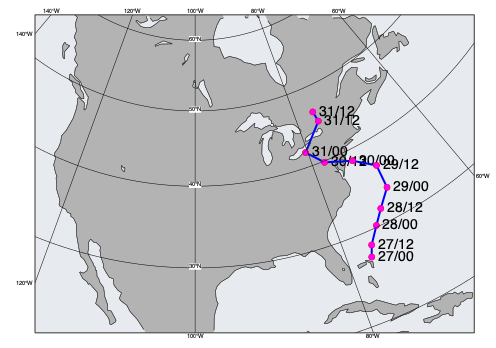
Limitations
Trackoffers a high-level interface and uses pre-defined settings, therefore it comes with certain limitations:
the date format must be yyyymmdd
the time format must be hh
the label format is hard-coded as dd/hh
it cannot be plotted with
plot()Note
If you would like to create a fully customised track plot from CSV data see the Storm track gallery example (it uses
read_table(),input_visualiser(),mgraph()andmsymb()to build the track).