Note
Click here to download the full example code
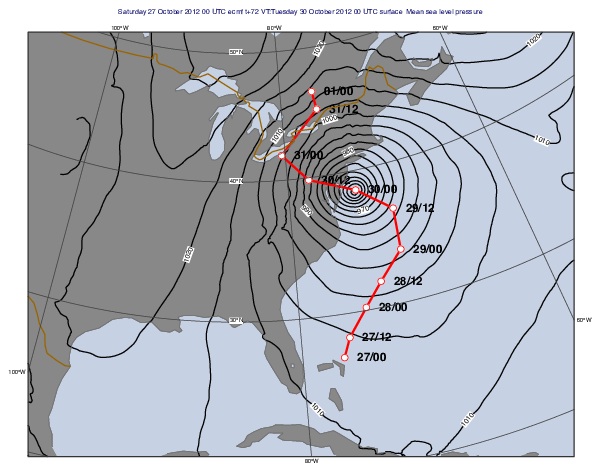
GRIB, CSV - Storm Track
# (C) Copyright 2017- ECMWF.
#
# This software is licensed under the terms of the Apache Licence Version 2.0
# which can be obtained at http://www.apache.org/licenses/LICENSE-2.0.
#
# In applying this licence, ECMWF does not waive the privileges and immunities
# granted to it by virtue of its status as an intergovernmental organisation
# nor does it submit to any jurisdiction.
#

import metview as mv

# read CSV file with the track positions and dates
filename = "sandy_track.txt"
if not mv.exist(filename):
    mv.gallery.load_dataset(filename)

tbl = mv.read_table(
    table_delimiter=" ",
    table_combine_delimiters="on",
    table_header_row=0,
    table_filename="sandy_track.txt",
)

# read track details into a set of vectors
val_date = mv.values(tbl, 0)
val_time = mv.values(tbl, 1)
val_lon = mv.values(tbl, 2)
val_lat = mv.values(tbl, 3)

# to plot text labels at each point, we will need to use the 'text' mode
# of msymb(). This requires associating each point with its text label, so we will
# generate values of 0,1,2,3,...,N-1 for the points and create an msymb() that
# maps each value to a generated date/time label.
val_idx = list(range(len(val_lat)))  # indexes: 0->N-1

# define date and time labels for track points
val_label = []
for i in range(len(val_date)):
    val_label.append(
        "   " + str(val_date[i])[6:8] + "/" + "{:02d}".format(int(val_time[i]))
    )

# define line and symbol properties
track_graph = mv.mgraph(
    graph_line_colour="red",
    graph_line_thickness=4,
    graph_symbol="on",
    graph_symbol_colour="white",
    graph_symbol_height=0.5,
    graph_symbol_marker_index=15,
    graph_symbol_outline="on",
    graph_symbol_outline_colour="red",
)

# define label properties
track_text = mv.msymb(
    legend="off",
    symbol_type="text",
    symbol_table_mode="advanced",
    symbol_advanced_table_selection_type="list",
    symbol_advanced_table_level_list=[*val_idx, val_idx[-1] + 1],
    symbol_advanced_table_text_list=val_label,
    symbol_advanced_table_text_font_size=0.5,
    symbol_advanced_table_text_font_style="bold",
    symbol_advanced_table_text_font_colour="black",
    symbol_advanced_table_text_display_type="right",
)

# create a visualiser for the track
track_vis = mv.input_visualiser(
    input_plot_type="geo_points",
    input_longitude_values=val_lon,
    input_latitude_values=val_lat,
    input_values=val_idx,
)

# read mslp forecast from grib file
filename = "sandy_mslp.grib"
if mv.exist(filename):
    g_mslp = mv.read(filename)
else:
    g_mslp = mv.gallery.load_dataset(filename)

# define mslp contouring
cont_mslp = mv.mcont(
    contour_line_thickness=2,
    contour_line_colour="black",
    contour_highlight="off",
    contour_level_selection_type="interval",
    contour_interval=5,
    grib_scaling_of_derived_fields="on",
)

# define coastline
coast = mv.mcoast(
    map_coastline_colour="RGB(0.4449,0.4414,0.4414)",
    map_coastline_resolution="low",
    map_coastline_land_shade="on",
    map_coastline_land_shade_colour="RGB(0.5333,0.5333,0.5333)",
    map_coastline_sea_shade="on",
    map_coastline_sea_shade_colour="RGB(0.7765,0.8177,0.8941)",
    map_boundaries="on",
    map_boundaries_colour="mustard",
    map_boundaries_thickness=2,
    map_grid_colour="RGB(0.2627,0.2627,0.2627)",
)

# define geographical view
view = mv.geoview(
    map_projection="polar_stereographic",
    map_area_definition="corners",
    area=[19.72, -98.59, 42.61, -47.28],
    map_vertical_longitude=-85,
    coastlines=coast,
)

# define the output plot file
mv.setoutput(mv.pdf_output(output_name="storm_track"))

# Plot the track and the mslp
mv.plot(view, g_mslp, cont_mslp, track_vis, track_text, track_graph)