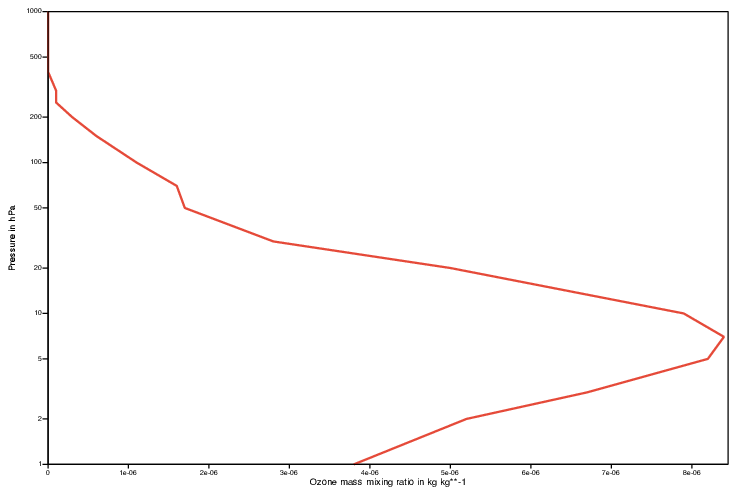
Cartesian View Curve with Logarithmic Y Axis

# (C) Copyright 2017- ECMWF.
#
# This software is licensed under the terms of the Apache Licence Version 2.0
# which can be obtained at http://www.apache.org/licenses/LICENSE-2.0.
#
# In applying this licence, ECMWF does not waive the privileges and immunities
# granted to it by virtue of its status as an intergovernmental organisation
# nor does it submit to any jurisdiction.
#

import metview as mv

# read the GRIB data into a fieldset
filename = "ozone_pl.grib"
if mv.exist(filename):
    g = mv.read(filename)
else:
    g = mv.gallery.load_dataset(filename)

# extract the values at a point, and the vertical levels
levels = mv.grib_get_double(g, "level")
ozone = mv.nearest_gridpoint(g, [-85, 0])

# define curve
vis_curve = mv.input_visualiser(input_x_values=ozone, input_y_values=levels)

# define curve style
gr_curve = mv.mgraph(
    graph_type="curve", graph_line_colour="coral", graph_line_thickness=4
)

# define a nice title for the x axis
# use object methods to get metadata, just to show the alternative
# to using functions
x_title = g[0].grib_get_string("name") + " in " + g[0].grib_get_string("units")
x_axis = mv.maxis(axis_title_text=x_title)

# define y axis title
y_title = "Pressure in hPa"
y_axis = mv.maxis(axis_title_text=y_title)

# define view, setting a log y axis
view = mv.cartesianview(
    x_automatic="off",
    x_min=0,
    x_max=max(ozone),
    y_automatic="on",
    y_axis_type="logarithmic",
    horizontal_axis=x_axis,
    vertical_axis=y_axis,
)

# define the output plot file
mv.setoutput(mv.pdf_output(output_name="cartesian_log_y_axis"))

# generate plot
mv.plot(view, vis_curve, gr_curve)