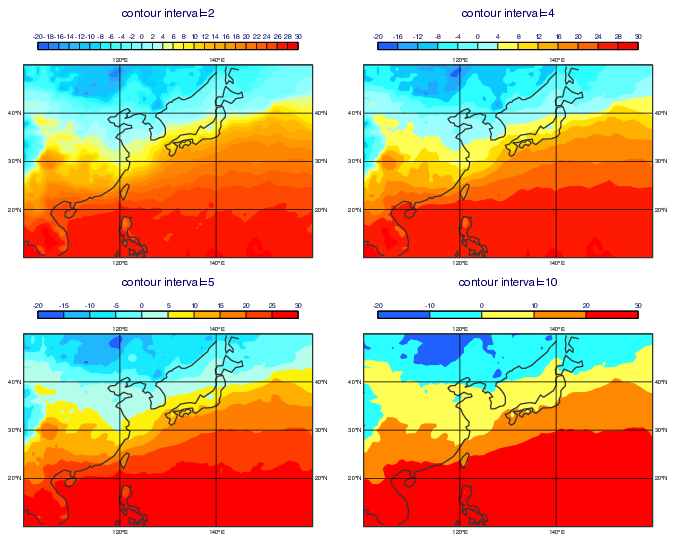
GRIB - Dynamic Contour Shading Palette

# (C) Copyright 2017- ECMWF.
#
# This software is licensed under the terms of the Apache Licence Version 2.0
# which can be obtained at http://www.apache.org/licenses/LICENSE-2.0.
#
# In applying this licence, ECMWF does not waive the privileges and immunities
# granted to it by virtue of its status as an intergovernmental organisation
# nor does it submit to any jurisdiction.
#

import metview as mv


# read the input grib file
filename = "2m_temperature.grib"
if mv.exist(filename):
    f = mv.read(filename)
else:
    f = mv.gallery.load_dataset(filename)


# define contour_shading using dynamic palette mode. We use 4 different
# contour intervals for the same palette and define a title for each.
intervals = [2, 4, 5, 10]

cont_lst = []
title_lst = []
for interval in intervals:
    # define contouring
    cont = mv.mcont(
        legend="on",
        contour="off",
        contour_level_selection_type="interval",
        contour_max_level=30,
        contour_min_level=-20,
        contour_interval=interval,
        contour_label="off",
        contour_shade="on",
        contour_shade_method="area_fill",
        contour_shade_colour_method="palette",
        contour_shade_palette_name="norway_blue_red_16",
        contour_shade_colour_list_policy="dynamic",
    )
    cont_lst.append(cont)

    # define title
    title = mv.mtext(
        text_lines=[f"contour interval={interval}", ""],
        text_font_size=0.5,
    )
    title_lst.append(title)

# define coastlines
coastlines = mv.mcoast(
    map_coastline_colour="charcoal",
    map_coastline_thickness=2,
)

# define geographical view
view = mv.geoview(
    map_area_definition="corners", area=[50, 100, 10, 160], coastlines=coastlines
)

# create a 2x2 plot layout with the defined geoview
dw = mv.plot_superpage(pages=mv.mvl_regular_layout(view, 2, 2, 1, 1, [5, 100, 15, 100]))

# define legend
legend = mv.mlegend(legend_text_font_size=0.3)

# define output
mv.setoutput(mv.pdf_output(output_name="dynamic_palette"))

# generate plot
gr = []
for i in range(4):
    gr.extend([dw[i], f, cont_lst[i], legend, title_lst[i]])

mv.plot(gr)