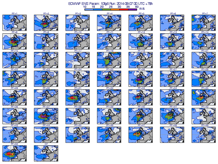
GRIB - ENS Stamp Map with Shared Legend and Title

# (C) Copyright 2017- ECMWF.
#
# This software is licensed under the terms of the Apache Licence Version 2.0
# which can be obtained at http://www.apache.org/licenses/LICENSE-2.0.
#
# In applying this licence, ECMWF does not waive the privileges and immunities
# granted to it by virtue of its status as an intergovernmental organisation
# nor does it submit to any jurisdiction.
#

import metview as mv


def _build_text_box(text, idx, rows, cols):
    """Build text box for an individual map"""

    # these params are setup for rows=8 cols=7. For other rows/cols
    # values the params HAVE TO BE ADJUSTED!!

    # positions are in cm and have to be adjusted manually!
    # x goes from left, y from top. We suppose the output is
    # A4 landscape!
    x_left = 0.9
    x_gap = 1
    x_width = 3.1
    x_offset = x_width / 2
    y_top = 19.08
    y_gap = 0.33
    y_width = 2.08
    y_offset = 0.1

    # figure out i, j index for the map. We suppose idx
    # starts at 0
    j = int(idx / cols)
    i = idx - j * cols

    # bottom centre of text box
    xp = x_left + i * x_gap + i * x_width + x_offset
    yp = y_top - j * y_gap - j * y_width - y_offset

    # box dimensions
    box_width = 2
    box_height = 1

    return mv.mtext(
        text_lines=[text],
        text_font_size=0.35,
        text_mode="positional",
        text_box_x_position=xp - box_width / 2,
        text_box_y_position=yp,
        text_box_x_length=box_width,
        text_box_y_length=box_height,
        text_justification="centre",
    )


# read ENS forecast
filename = "wgust_ens.grib"
if mv.exist(filename):
    g = mv.read(filename)
else:
    g = mv.gallery.load_dataset(filename)

# filter out a timestep
wg = mv.read(data=g, step=78)

# define contour shading
wgust_shade = mv.mcont(
    legend="off",
    contour_line_colour="navy",
    contour_highlight="off",
    contour_level_selection_type="level_list",
    contour_level_list=[10, 15, 20, 25, 30, 35, 50],
    contour_label="off",
    contour_shade="on",
    contour_shade_colour_method="list",
    contour_shade_method="area_fill",
    contour_shade_colour_list=[
        "sky",
        "greenish_blue",
        "avocado",
        "orange",
        "orangish_red",
        "violet",
    ],
)

# define coastline
coast = mv.mcoast(
    map_coastline_land_shade="on",
    map_coastline_land_shade_colour="grey",
    map_coastline_sea_shade="on",
    map_coastline_sea_shade_colour="RGB(0.8944,0.9086,0.933)",
    map_coastline_thickness=2,
    map_boundaries="on",
    map_boundaries_colour="charcoal",
    map_label="off",
    map_grid_colour="RGB(0.6, 0.6, 0.6)",
    map_grid_longitude_increment=10,
)

# width of an A4 landscape page in cm
pw = 29.7

# number of map rows and columns
# Warning: when changing these numbers _build_text_box() has to be adjusted!
rows_num = 8
cols_num = 7

# define map view
view = mv.geoview(
    map_area_definition="corners", area=[40, -20, 60, 10], coastlines=coast
)

# define layout for the ENS plots. We will leave the first row empty, we use
# this space for the title and legend
pages = mv.mvl_regular_layout(view, cols_num, rows_num, 1, 1, [8, 100, 2, 98])

# ---------------------------------------------
# define positional title at the top
# ---------------------------------------------

# we want to show a shared title at the top of the page. The space is
# is simple not enough above the maps to display this amount of information.

# create an annotation view covering the whole page area (dimensions are in %).
# It is just a placeholder and its only purpose is to hold custom positional
# mtext objects.
title_view = mv.annotationview()

# create the page (dimensions are in %) holding the annotation view. For simplicity
# it covers the whole plot area
title_page = mv.plot_page(top=0, bottom=100, left=0, right=100, view=title_view)

pages.append(title_page)

# create a positional title to be added to the annotation view.
# Note: its coordinates are in cm! x is measured from the left side
# of the parent page (e.i. title_page), while y is measured from the bottom
# of the parent page!

bdate = mv.base_date(wg[0])
param_name = mv.grib_get_string(wg[0], "shortName")
step = mv.grib_get_string(wg[0], "step")
shared_title = mv.mtext(
    text_lines="ECMWF ENS Param: {} Run: {} +{}h".format(
        param_name, bdate.strftime("%Y-%m-%d %H UTC"), step
    ),
    text_font_size=0.5,
    text_mode="positional",
    text_box_x_position=pw / 2 - 20 / 2,
    text_box_y_position=20.2,
    text_box_x_length=20,
    text_box_y_length=1.5,
    text_justification="centre",
)

# ----------------------------------------------
# define positional shared legend at the top
# ----------------------------------------------

# we do not want to display the legend for each plot (since the space is
# confined) but want to show only one legend atop just below the main page title.
# Since the legend is only generated when data is plotted into a view, we will
# create an "invisible" geo view and properly adjust it so that the legend can
# appear at the desired position.

# create an empty coastlines
empty_coast = mv.mcoast(map_coastline="off", map_grid="off", map_label="off")

# create a geoview
legend_view = mv.geoview(
    page_frame="off",
    subpage_frame="off",
    coastlines=empty_coast,
    subpage_x_position=40,
    subpage_y_position=65,
    subpage_x_length=20,
    subpage_y_length=20,
)

# create a page (dimensions are in %) holding the view. It is positioned at the
# top of the A4 superpage
legend_page = mv.plot_page(top=0, bottom=20, left=0, right=100, view=legend_view)

pages.append(legend_page)

# create a field to be plotted into the view. It should only contain missing values,
# since we do not want to generate any result
empty_fld = mv.bitmap(wg[0] * 0, 0)

# define the contouring. It is the same that we defined for g but the
# legend has to be enabled now!
empty_cont = mv.mcont(**wgust_shade, legend="on")

# define an empty title
empty_title = mv.mtext(text_line_count=0)

# define the legend. Note: its coordinates are in cm! x is measured
# from the left side of the parent page (legend_page), while y is measured from
# the bottom of the parent page!
shared_legend = mv.mlegend(
    legend_box_mode="positional",
    legend_text_font_size=0.45,
    legend_box_x_position=11,
    legend_box_y_position=2.8,
    legend_box_x_length=10,
    legend_box_y_length=0.4,
    legend_units_text="m/s",
    legend_title="on",
    legend_title_text="m/s",
    legend_title_position="right",
)

# create the final layout
dw = mv.plot_superpage(pages=pages)

# define the output plot file
mv.setoutput(mv.pdf_output(output_name="ens_stamp_shared_legend_title"))

# generate plot
pl_lst = []

# perturbed forecasts
for i in range(1, 51):
    f = mv.read(data=wg, type="pf", number=i)
    dw_index = i - 1

    # map plot
    pl_lst.append([dw[dw_index], f, wgust_shade, mv.mtext(text_line_count=0)])

    # add positional title (will be added to title_view!)
    title = _build_text_box("PF=" + str(i), dw_index, rows_num, cols_num)
    pl_lst.append([dw[-2], f, wgust_shade, title])

# control forecast - plot
dw_index = 50
f = mv.read(data=wg, type="cf")
pl_lst.append([dw[dw_index], f, wgust_shade, mv.mtext(text_line_count=0)])

# control forecast - add positional title (will be added to title_view!)
title = _build_text_box("CF", dw_index, rows_num, cols_num)
pl_lst.append([dw[-2], f, wgust_shade, title])

# shared title
pl_lst.extend([dw[-2], shared_title])

# shared legend
pl_lst.extend([dw[-1], empty_fld, empty_cont, shared_legend, empty_title])

mv.plot(pl_lst)