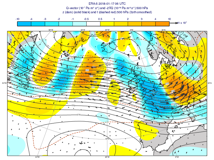
GRIB - Q-vector

# (C) Copyright 2017- ECMWF.
#
# This software is licensed under the terms of the Apache Licence Version 2.0
# which can be obtained at http://www.apache.org/licenses/LICENSE-2.0.
#
# In applying this licence, ECMWF does not waive the privileges and immunities
# granted to it by virtue of its status as an intergovernmental organisation
# nor does it submit to any jurisdiction.
#

import metview as mv

# Note: at least Metview version 5.17.0 is required for this example

# getting data
use_cds = False

filename = "friederike.grib"

# getting data from CDS
if use_cds:
    import cdsapi

    c = cdsapi.Client()
    c.retrieve(
        "reanalysis-era5-pressure-levels",
        {
            "product_type": "reanalysis",
            "format": "grib",
            "variable": [
                "geopotential",
                "temperature",
                "u_component_of_wind",
                "v_component_of_wind",
            ],
            "pressure_level": ["1000", "925", "850", "700", "600", "500", "400", "300"],
            "year": "2018",
            "month": "01",
            "day": "17",
            "time": "06:00",
            "area": [
                90,
                -100,
                10,
                80,
            ],
        },
        filename,
    )
    g = mv.read(filename)
# reading data from file or getting from data server
else:
    if mv.exist(filename):
        g = mv.read(filename)
    else:
        g = mv.gallery.load_dataset(filename)

# get fields on 500 hPa and interpolate onto a 1x1 degree grid
grid = [1, 1]
level = 500
t = mv.read(data=g, param="t", levelist=level, grid=grid)
z = mv.read(data=g, param="z", levelist=level, grid=grid)

# smooth the fields used for the Q vector computations to get only
# large scale synoptic features. Otherwise the results would be
# extremely noisy
t = t.smooth_n_point(n=9, repeat=20)
z = z.smooth_n_point(n=9, repeat=20)

# compute the Q vector
qv = mv.q_vector(t, z, static_stability=2e-6)

# compute the right hand side term in the QG omega equation
div_q = -2 * mv.divergence(qv[0], qv[1])

# scale fields for plotting
qv = qv * 1e7
div_q = div_q * 1e12

# shading for the divergence term
cont_dq = mv.mcont(
    legend="on",
    contour="off",
    contour_level_selection_type="level_list",
    contour_level_list=[-10, -4, -3, -2, -1, -0.5, 0.5, 1, 2, 3, 4, 10],
    contour_label="off",
    contour_shade="on",
    contour_shade_colour_method="palette",
    contour_shade_method="area_fill",
    contour_shade_palette_name="eccharts_cyan_orange_11",
    contour_shade_colour_list_policy="dynamic",
)

# vector plotting style for the Q vector
style_qv = mv.mwind(
    wind_thinning_factor=2,
    wind_arrow_colour="charcoal",
    wind_arrow_thickness=2,
    wind_arrow_unit_velocity=11,
    legend="on",
    wind_legend_text=" 11 x 10⁻⁷",
)

# geopotential style
cont_z = mv.mcont(
    contour_line_thickness=2,
    contour_line_colour="charcoal",
    contour_highlight_colour="charcoal",
    contour_highlight="off",
    contour_level_selection_type="interval",
    contour_interval=4,
    grib_scaling_of_derived_fields="on",
)

# temperature style
cont_t = mv.mcont(
    contour_line_colour="rust",
    contour_line_thickness=2,
    contour_line_style="dash",
    contour_highlight="off",
    contour_level_selection_type="interval",
    contour_interval=4,
    grib_scaling_of_derived_fields="on",
)

# define view
coastlines = mv.mcoast(
    map_coastline_resolution="medium",
    map_coastline_land_shade="on",
    map_coastline_land_shade_colour="RGB(0.8169,0.8066,0.8066)",
    map_grid_colour="RGB(0.6039,0.6039,0.6039)",
)

view = mv.geoview(
    map_projection="polar_stereographic",
    map_area_definition="centre",
    map_vertical_longitude=-20,
    map_centre_latitude=52,
    map_centre_longitude=-20,
    map_scale=2.5e7,
    coastlines=coastlines,
)

# define title
vdate = mv.valid_date(div_q[0])

title = mv.mtext(
    text_lines=[
        "ERA-5  {}".format(vdate.strftime("%Y-%m-%d %H UTC")),
        f"Q-vector (10⁻⁷ Pa m⁻¹ s⁻¹) and -2∇Q (10⁻¹² Pa m⁻² s⁻¹) {level} hPa",
        f"z (dam) (solid black) and t (dashed red) {level} hPa (both smoothed)",
        "",
    ],
    text_font_size=0.45,
)

# define legend
legend = mv.mlegend(legend_text_font_size=0.4)

# define the output plot file
mv.setoutput(mv.pdf_output(output_name="q_vector"))

# generate plot
mv.plot(view, div_q, cont_dq, t, cont_t, z, cont_z, qv, style_qv, legend, title)