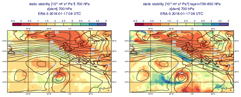
GRIB - Static Stability

# (C) Copyright 2017- ECMWF.
#
# This software is licensed under the terms of the Apache Licence Version 2.0
# which can be obtained at http://www.apache.org/licenses/LICENSE-2.0.
#
# In applying this licence, ECMWF does not waive the privileges and immunities
# granted to it by virtue of its status as an intergovernmental organisation
# nor does it submit to any jurisdiction.
#

import metview as mv

# Note: at least Metview version 5.17.0 is required for this example

# getting data
use_cds = False

filename = "friederike.grib"

# getting data from CDS
if use_cds:
    import cdsapi

    c = cdsapi.Client()
    c.retrieve(
        "reanalysis-era5-pressure-levels",
        {
            "product_type": "reanalysis",
            "format": "grib",
            "variable": [
                "geopotential",
                "temperature",
                "u_component_of_wind",
                "v_component_of_wind",
            ],
            "pressure_level": ["1000", "925", "850", "700", "600", "500", "400", "300"],
            "year": "2018",
            "month": "01",
            "day": "17",
            "time": "06:00",
            "area": [
                90,
                -100,
                10,
                80,
            ],
        },
        filename,
    )
    f = mv.read(filename)
# reading data from file or getting from data server
else:
    if mv.exist(filename):
        f = mv.read(filename)
    else:
        f = mv.gallery.load_dataset(filename)


# get z data (only used for plotting)
z = f.select(shortName="z", level=700)

# compute static stability on each level and scale results
# for plotting
t = f.select(shortName="t", level=[850, 700, 500])
s = mv.static_stability(t)
s = s * 1e6

# extract results on 700 hPa
s1 = s.select(level=700)

# compute static stability for a layer and scale results
# for plotting
t = f.select(shortName="t", level=[850, 700])
s = mv.static_stability(t, layer=True)
s2 = s * 1e6

# define contour shading for static stability
cont_sigma = mv.mcont(
    legend="on",
    contour="off",
    contour_level_selection_type="interval",
    contour_max_level=5,
    contour_shade_min_level=-0.5,
    contour_interval=0.5,
    contour_label="off",
    contour_shade="on",
    contour_shade_colour_method="palette",
    contour_shade_method="area_fill",
    contour_shade_palette_name="colorbrewer_Spectral",
    contour_shade_colour_list_policy="dynamic",
    contour_shade_colour_reverse_list="on",
)

# define contouring for geopotential
cont_z = mv.mcont(
    contour_line_thickness=2,
    contour_line_colour="charcoal",
    contour_highlight="off",
    contour_highlight_colour="charcoal",
    contour_highlight_thickness=4,
    contour_level_selection_type="interval",
    contour_interval=5,
    contour_label_height=0.3,
    grib_scaling_of_derived_fields="on",
)

# define coastlines
coast = mv.mcoast(map_coastline_colour="chestnut", map_coastline_thickness=2)

# define geographical view
view = mv.geoview(area_mode="name", area_name="north_atlantic", coastlines=coast)
view = mv.geoview(
    map_area_definition="corners", area=[70, -60, 10, 40], coastlines=coast
)

# define layout
page_0 = mv.plot_page(top=20, bottom=80, right=50, view=view)
page_1 = mv.plot_page(top=20, bottom=80, left=50, right=100, view=view)
dw = mv.plot_superpage(page=[page_0, page_1])

# define title
vdate = mv.base_date(z)
title1 = mv.mtext(
    text_lines=[
        "static stability [10⁻⁶ m² s⁻² Pa⁻²] 700 hPa",
        "z[dam] 700 hPa",
        "ERA-5 {}".format(vdate.strftime("%Y-%m-%d %H UTC")),
        "",
    ],
    text_font_size=0.5,
)

title2 = mv.mtext(
    text_lines=[
        "static stability [10⁻⁶ m² s⁻² Pa⁻²] layer=700-850 hPa",
        "z[dam] 700 hPa",
        "ERA-5 {}".format(vdate.strftime("%Y-%m-%d %H UTC")),
        "",
    ],
    text_font_size=0.5,
)

# define legend
legend = mv.mlegend(legend_text_font_size=0.35)

# define the output plot file
mv.setoutput(mv.pdf_output(output_name="static_stability"))

# generate plot
mv.plot(
    dw[0],
    s1,
    cont_sigma,
    z,
    cont_z,
    title1,
    legend,
    dw[1],
    s2,
    cont_sigma,
    z,
    cont_z,
    title2,
    legend,
)