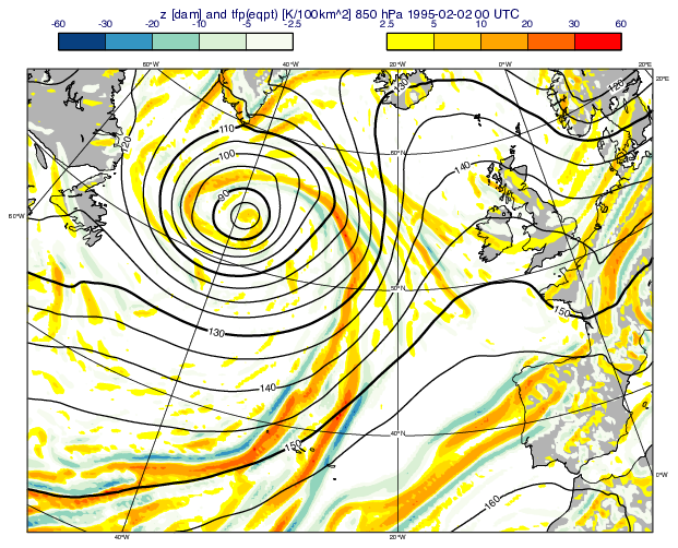
GRIB - Thermal Front Parameter

# (C) Copyright 2017- ECMWF.
#
# This software is licensed under the terms of the Apache Licence Version 2.0
# which can be obtained at http://www.apache.org/licenses/LICENSE-2.0.
#
# In applying this licence, ECMWF does not waive the privileges and immunities
# granted to it by virtue of its status as an intergovernmental organisation
# nor does it submit to any jurisdiction.
#

import metview as mv

# getting data
use_cds = False

filename = "tfp_era5.grib"

# getting forecast data from CDS
if use_cds:
    import cdsapi

    c = cdsapi.Client()
    c.retrieve(
        "reanalysis-era5-pressure-levels",
        {
            "product_type": "reanalysis",
            "format": "grib",
            "variable": [
                "geopotential",
                "specific_humidity",
                "temperature",
            ],
            "pressure_level": [
                "850",
            ],
            "year": "1995",
            "month": "02",
            "day": "02",
            "time": "00:00",
            "area": [
                90,
                -100,
                20,
                40,
            ],
        },
        filename,
    )
    g = mv.read(filename)
# read data from file
else:
    if mv.exist(filename):
        g = mv.read(filename)
    else:
        g = mv.gallery.load_dataset(filename)

# get fields on 850 hPa
level = 850
t = mv.read(data=g, param="t", levelist=level)
q = mv.read(data=g, param="q", levelist=level)
z = mv.read(data=g, param="z", levelist=level)

# the thermal front parameter (tfp) will be computed for
# equivalent potential temperature. We compute eqpt from t and q.
eqpt = mv.eqpott_p(temperature=t, humidity=q)

# compute the gradient
gr = mv.gradient(eqpt)

# compute the norm of the gradient and bitmap it (=set missing values)
# for values close to zero. We have to do it because the norm will appear
# in the denominator and we have to avoid division by zero.
ngr = mv.sqrt(gr[0] ** 2 + gr[1] ** 2)
ngr = ngr * mv.bitmap(ngr > 1e-18, 0)

# the second term in the tfp is the normalised gradient
t_2 = mv.merge(gr[0] / ngr, gr[1] / ngr)

# the first term in the tfp is the gradient of the negative of the norm
t_1 = mv.gradient(-ngr)

# the tfp is the scalar product of the two terms
tfp = t_1[0] * t_2[0] + t_1[1] * t_2[1]

# define contouring
pos_tfp = mv.mcont(
    legend="on",
    contour="off",
    contour_level_selection_type="level_list",
    contour_level_list=[2.5, 5, 10, 20, 30, 60],
    contour_label="off",
    contour_shade="on",
    contour_shade_colour_method="palette",
    contour_shade_method="area_fill",
    contour_shade_palette_name="eccharts_yellow_red_5",
)

neg_tfp = mv.mcont(
    legend="on",
    contour="off",
    contour_level_selection_type="level_list",
    contour_level_list=[-60, -30, -20, -10, -5, -2.5],
    contour_label="off",
    contour_shade="on",
    contour_shade_colour_method="palette",
    contour_shade_method="area_fill",
    contour_shade_palette_name="colorbrewer_GnBu_5",
)

cont_z = mv.mcont(contour_automatic_setting="ecmwf", legend="off")

# define coastlines
coast = mv.mcoast(map_coastline_land_shade="on", map_coastline_land_shade_colour="grey")

# define the geographical view
view = mv.geoview(
    map_projection="polar_stereographic",
    map_area_definition="corners",
    area=[28.51, -46.05, 59.27, 20.89],
    map_vertical_longitude=-20,
    coastlines=coast,
)

# define title
vdate = mv.valid_date(z)
title = mv.mtext(
    text_lines="z [dam] and tfp(eqpt) [K/100km^2] {} hPa {}".format(
        level, vdate.strftime("%Y-%m-%d %H UTC")
    ),
    text_font_size=0.5,
)

# define legend
legend = mv.mlegend(legend_text_font_size=0.4)

# define output
mv.setoutput(mv.pdf_output(output_name="thermal_front_parameter"))

# generate plot. The tfp is scaled from K/m2 -> K/100km2 units
mv.plot(view, tfp * 1e10, neg_tfp, pos_tfp, z, cont_z, title, legend)