thermo_parcel_path

thermo_parcel_path(profile, mode='mucape', virtual=True, start_t=None, start_td=None, start_p=None, top_p=None, bottom_p=None, layer_depth=None, stop_at_el=False, comp_top=False)

thermo_parcel_path(t, td, p, **kwargs)

Computes the path of an ascending thermodynamic parcel with the given start condition for the given vertical profile.

Parameters

profile (thermo_bufr() or thermo_grib()) – profile data extracted from a Fieldset or Bufr for a thermodynamic diagram
t (ndarray) – temperature profile (°C)
td (ndarray) – dewpoint temperature profile (°C)
p (ndarray) – pressure profile (hPa)
mode (str) – the start condition mode. The possible values are “surface”, “custom”, “ml”, “ml50”, “ml100” and “mucape” (see below for details)
virtual (bool) – enables the virtual temperature correction. Default is True.
start_t (number) – the start temperature (°C) of the parcel when mode is “custom”
start_td (number) – the start dewpoint (°C) of the parcel when mode is “custom”
start_p (number) – the start pressure (hPa) of the parcel when mode is “custom”
top_p (number) – the top pressure (hPa) of the start layer when mode is “ml” or “mucape”. Cannot be used together with layer_depth.
bottom_p (number) – the bottom pressure (hPa) of the start layer when mode is “ml” or “mucape”. When it is None the pressure layer starts at the surface.
layer_depth (number) – the depth of the start layer (hPa) when mode is “ml” or “mucape”. Cannot be used together with top_p. When none of top_p, bottom_p and layer_depth is specified, it is implicitly set to 100 when mode is “ml” and to 300 when mode is “mucape”.
stop_at_el (bool) – makes all parcel computations stop at the Equilibrium Level (EL). Default is False.
comp_top (bool) – enables the computation of the Cloud Top Level (TOP). Default is False. Ignored when stop_at_el is enabled.

Return type

dict

Returns a dict containing all the data to plot the parcel path, buoyancy areas and related data into a thermodynamic diagram.

All the input values must be specified in °C (temperature) and hPa (pressure) units. The actual start condition is determined by mode:

“surface”: the parcel ascends from the surface, i.e. the lowest point of the profile. E.g.:
mv.thermo_parcel_path(prof, mode="surface")

“custom”: the parcel ascends from a given temperature, dewpoint and pressure. E.g.:

mv.thermo_parcel_path(prof, mode="custom",
    start_t=27.2,
    start_td=21.8,
    start_p=998)

When no start_t or start_td is specified the parcel started from level start_p on the profile.

“ml”: the parcel ascends from the following mean start condition in a given layer:
- temperature: determined from the mean potential temperature of the layer
- dew point: the mean value in the layer
- pressure: the surface value

The layer is specified with the combination of top_p, bottom_p, layer_depth. When bottom_p is None the pressure layer starts at the surface. E.g.:
mv.thermo_parcel_path(prof, mode="ml", layer_depth=150)
When none of top_p, bottom_p and layer_depth is specified, layer_depth is implicitly set to 100. E.g.
# these calls are equivalent
mv.thermo_parcel_path(prof, mode="ml", layer_depth=100)
mv.thermo_parcel_path(prof, mode="ml")

“ml50”: the parcel ascends from the mean start condition in the lowest 50 hPa layer above the surface. The start condition is determined similarly to “ml”.
“ml100”: the parcel ascends from the mean start condition in the lowest 100 hPa layer at the surface. The start condition is determined similarly to “ml”.
“mucape”: the parcel ascends from the most unstable condition. This is the default mode. To determine “mucape”, a parcel is started from all the points along the profile in the specified pressure layer. The start level of the parcel that results in the highest CAPE value will define the most unstable start condition. The layer is specified with the combination of top_p, bottom_p, layer_depth. When no bottom_p is specified the pressure layer starts at the surface. E.g.
mv.thermo_parcel_path(prof, mode="mucape", layer_depth=200)

When none of top_p, bottom_p and layer_depth is specified, layer_depth is implicitly set to 300. E.g.

# these calls are equivalent
mv.thermo_parcel_path(prof, mode="mucape", layer_depth=300)
mv.thermo_parcel_path(prof, mode="mucape")
mv.thermo_parcel_path(prof)

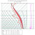
thermo_parcel_path() returns a dict containing all the parameters related to the ascent of the parcel. The members of this dict are as follows (temperature values are in °C and pressure values are in hPa) :

“path”: path of the parcel. It is itself a dict with two members: t and p, both containing a list of values.
“area”: positive and negative buoyancy areas between the parcel path and the profile. It is a list of dictionaries describing the areas.
“cape”: value of the CAPE (Convective Available Potential Energy) (J/kg). It is always a positive value or zero if it cannot be determined.
“cin”: value the CIN (Convective Inhibition) (J/kg). It is always a positive value or zero if it cannot be determined.
“li”: the Lifted Index (K)
“lcl”: Lifted Condensation Level. It is a dict with two members: t and p. If no LCL exists it is set to None.
“lfc”: Level of Free Convection. It is a dict with two members: t and p. If no LFC exists it is set to None.
“el”: Equilibrium Level. It is a dict with two members: t and p. If no EL exists it is set to None.
“top”: Cloud Top Level. It is a dict with two members: t and p. If no TOP exists it is set to None.
“start”: start conditions of the parcel with four members: mode, t, td and p.

Note

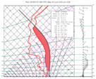
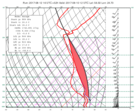
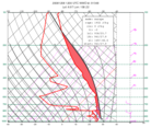
The parcel method is based on the path of a hypothetical ascending air parcel, which can be best represented on thermodynamic diagrams.

The parcel starts ascending dry adiabatically until it reaches saturation at the LCL (Lifted Condensation Level). Above the LCL thermo_parcel_path() assumes a pseudo-adiabatic ascent (all condensate is removed as soon as it forms) determined by the saturation equivalent potential temperature at the LCL, which is invariant along a pseudo-adiabat. The (saturation)equivalent potential temperature is computed by Eq (39) from [Bolton1980].

By default, the virtual temperature correction is applied (virtual is True) and the temperature in both the environment and parcel profiles are replaced with the virtual_temperature().

Once its done the intersections of the environment and parcel virtual temperature profiles are determined to define the positive and negative buoyancy areas. In a positive area the parcel is warmer, while in a negative area it is colder than its environment. In the simplest case there is only one positive area above the LCL bounded by the LFC (Level of Free Convection) at the bottom and the EL (Equilibrium Level) at the top. However, in practice there can be several positive and negative areas above the LCL and thermo_parcel_path() makes the following choice for the computations:

the LFC is the bottom of the topmost positive area

the EL is the top of the topmost positive area

CAPE (Convective Available Potential Energy) is computed as the integral of the positive buoyancy between the LCL and EL, while CIN (Convective Inhibition) is the integral of the negative buoyancy between the start level and the LFC:

\[ \begin{align}\begin{aligned}CAPE = - R_{d} \int_{p_{LCL}}^{p_{EL}} max(T_{v,parcel} - T_{v,env}, 0) dlog(p)\\ CIN = R_{d} \int_{p_{START}}^{p_{LFC}} min(T_{v,parcel} - T_{v,env}, 0) dlog(p)\end{aligned}\end{align} \]

where \(R_{d}\) is the specific gas constant for dry air (287.058 J/(kg K)).

LI (Lifted index) is the difference between the virtual temperature of the environment and the parcel at 500 hPa.