Try this notebook in ![]() .
.
Slicing and dicing GRIB data
Terminology
A GRIB file consists of a sequence of self-contained GRIB messages. A GRIB file is represented as a Fieldset object in Metview. Each message contains the data for a single field, e.g. a single parameter generated at a single time at a single level for a single forecast step. A field contains a set of gridpoints geographically distributed in some way, plus metadata such as the parameter, the generation time, the forecast step and the centre that generated the data. A field may be plotted on a map, and a Fieldset may be plotted as an animation on a map.
Setting up
[3]:
import numpy as np
import metview as mv
[4]:
# not strictly necessary to tell Metview that we're running in a Jupyter notebook,
# but we will call this function so that we can specify a larger font size
mv.setoutput('jupyter', output_width=700, output_font_scale=1.5)
Reading and inspecting the data
[81]:
# get the data - if not already on disk then download
filename = "grib_to_be_sliced.grib"
if not mv.exist(filename):
    data = mv.gallery.load_dataset(filename)
else:
    data = mv.read('grib_to_be_sliced.grib')
print(data)
Fieldset (191 fields)
[6]:
# get an overview of the data in the GRIB file
data.describe()
[6]:
| parameter | typeOfLevel | level | date | time | step | number | paramId | class | stream | type | experimentVersionNumber |
|---|---|---|---|---|---|---|---|---|---|---|---|
| 2t | surface | 0 | 20220608 | 1200 | 0,6,... | 0 | 167 | od | oper | fc | 0001 |
| lsm | surface | 0 | 20220608 | 1200 | 0 | 0 | 172 | od | oper | fc | 0001 |
| q | isobaricInhPa | 100,150,... | 20220608 | 1200 | 0 | 0 | 133 | od | oper | fc | 0001 |
| r | isobaricInhPa | 100,150,... | 20220608 | 1200 | 0 | 0 | 157 | od | oper | fc | 0001 |
| t | isobaricInhPa | 100,150,... | 20220608 | 1200 | 0,6,... | 0 | 130 | od | oper | fc | 0001 |
| trpp | tropopause | 0 | 20220608 | 1200 | 0 | None | 228045 | od | oper | fc | 0001 |
| z | isobaricInhPa | 100,150,... | 20220608 | 1200 | 0 | 0 | 129 | od | oper | fc | 0001 |
[85]:
# dive into a specific parameter
data.describe('r')
[85]:
| shortName | r |
|---|---|
| name | Relative humidity |
| paramId | 157 |
| units | % |
| typeOfLevel | isobaricInhPa |
| level | 100,150,200,250,300,400,500,700,850,925,1000 |
| date | 20220608 |
| time | 1200 |
| step | 0 |
| class | od |
| stream | oper |
| type | fc |
| experimentVersionNumber | 0001 |
[8]:
data.describe('z')
[8]:
| shortName | z |
|---|---|
| name | Geopotential |
| paramId | 129 |
| units | m**2 s**-2 |
| typeOfLevel | isobaricInhPa |
| level | 100,150,200,250,300,400,500,700,850,925,1000 |
| date | 20220608 |
| time | 1200 |
| step | 0 |
| class | od |
| stream | oper |
| type | fc |
| experimentVersionNumber | 0001 |
[9]:
data.describe('t')
[9]:
| shortName | t |
|---|---|
| name | Temperature |
| paramId | 130 |
| units | K |
| typeOfLevel | isobaricInhPa |
| level | 100,150,200,250,300,400,500,700,850,925,1000 |
| date | 20220608 |
| time | 1200 |
| step | 0,6,12,18,24,30,36,42,48,54,60,66,72 |
| class | od |
| stream | oper |
| type | fc |
| experimentVersionNumber | 0001 |
[10]:
data.describe('lsm')
[10]:
| shortName | lsm |
|---|---|
| name | Land-sea mask |
| paramId | 172 |
| units | (0 - 1) |
| typeOfLevel | surface |
| level | 0 |
| date | 20220608 |
| time | 1200 |
| step | 0 |
| class | od |
| stream | oper |
| type | fc |
| experimentVersionNumber | 0001 |
[83]:
# similar to grib_ls on the command line - list all the fields
# - just print the first 20 - remove the [:20] to print all fields
data[:20].ls()
[83]:
| centre | shortName | typeOfLevel | level | dataDate | dataTime | stepRange | dataType | number | gridType | |
|---|---|---|---|---|---|---|---|---|---|---|
| Message | ||||||||||
| 0 | ecmf | 2t | surface | 0 | 20220608 | 1200 | 0 | fc | 0 | reduced_gg |
| 1 | ecmf | 2t | surface | 0 | 20220608 | 1200 | 6 | fc | 0 | reduced_gg |
| 2 | ecmf | 2t | surface | 0 | 20220608 | 1200 | 12 | fc | 0 | reduced_gg |
| 3 | ecmf | 2t | surface | 0 | 20220608 | 1200 | 18 | fc | 0 | reduced_gg |
| 4 | ecmf | 2t | surface | 0 | 20220608 | 1200 | 24 | fc | 0 | reduced_gg |
| 5 | ecmf | 2t | surface | 0 | 20220608 | 1200 | 30 | fc | 0 | reduced_gg |
| 6 | ecmf | 2t | surface | 0 | 20220608 | 1200 | 36 | fc | 0 | reduced_gg |
| 7 | ecmf | 2t | surface | 0 | 20220608 | 1200 | 42 | fc | 0 | reduced_gg |
| 8 | ecmf | 2t | surface | 0 | 20220608 | 1200 | 48 | fc | 0 | reduced_gg |
| 9 | ecmf | 2t | surface | 0 | 20220608 | 1200 | 54 | fc | 0 | reduced_gg |
| 10 | ecmf | 2t | surface | 0 | 20220608 | 1200 | 60 | fc | 0 | reduced_gg |
| 11 | ecmf | 2t | surface | 0 | 20220608 | 1200 | 66 | fc | 0 | reduced_gg |
| 12 | ecmf | 2t | surface | 0 | 20220608 | 1200 | 72 | fc | 0 | reduced_gg |
| 13 | ecmf | lsm | surface | 0 | 20220608 | 1200 | 0 | fc | 0 | reduced_gg |
| 14 | ecmf | trpp | tropopause | 0 | 20220608 | 1200 | 0 | fc | None | reduced_gg |
| 15 | ecmf | z | isobaricInhPa | 1000 | 20220608 | 1200 | 0 | fc | 0 | reduced_gg |
| 16 | ecmf | r | isobaricInhPa | 1000 | 20220608 | 1200 | 0 | fc | 0 | reduced_gg |
| 17 | ecmf | q | isobaricInhPa | 1000 | 20220608 | 1200 | 0 | fc | 0 | reduced_gg |
| 18 | ecmf | z | isobaricInhPa | 925 | 20220608 | 1200 | 0 | fc | 0 | reduced_gg |
| 19 | ecmf | r | isobaricInhPa | 925 | 20220608 | 1200 | 0 | fc | 0 | reduced_gg |
Field selection
Field selection through indexing
[12]:
# select the first field (0-based indexing)
print(data[0])
data[0].ls()
Fieldset (1 field)
[12]:
| centre | shortName | typeOfLevel | level | dataDate | dataTime | stepRange | dataType | gridType | |
|---|---|---|---|---|---|---|---|---|---|
| Message | |||||||||
| 0 | ecmf | 2t | surface | 0 | 20220608 | 1200 | 0 | fc | reduced_gg |
[13]:
# select the fourth field (0-based indexing)
data[3].ls()
[13]:
| centre | shortName | typeOfLevel | level | dataDate | dataTime | stepRange | dataType | gridType | |
|---|---|---|---|---|---|---|---|---|---|
| Message | |||||||||
| 0 | ecmf | 2t | surface | 0 | 20220608 | 1200 | 18 | fc | reduced_gg |
[14]:
# select the last field
data[-1].ls()
[14]:
| centre | shortName | typeOfLevel | level | dataDate | dataTime | stepRange | dataType | gridType | |
|---|---|---|---|---|---|---|---|---|---|
| Message | |||||||||
| 0 | ecmf | t | isobaricInhPa | 100 | 20220608 | 1200 | 72 | fc | reduced_gg |
[15]:
# index with numpy array
indices = np.array([1, 46, 27, 180])
data[indices].ls()
[15]:
| centre | shortName | typeOfLevel | level | dataDate | dataTime | stepRange | dataType | gridType | |
|---|---|---|---|---|---|---|---|---|---|
| Message | |||||||||
| 0 | ecmf | 2t | surface | 0 | 20220608 | 1200 | 6 | fc | reduced_gg |
| 1 | ecmf | r | isobaricInhPa | 100 | 20220608 | 1200 | 0 | fc | reduced_gg |
| 2 | ecmf | z | isobaricInhPa | 500 | 20220608 | 1200 | 0 | fc | reduced_gg |
| 3 | ecmf | t | isobaricInhPa | 1000 | 20220608 | 1200 | 72 | fc | reduced_gg |
Field selection through slicing
[16]:
# select fields 4 to 7
data[4:8].ls()
[16]:
| centre | shortName | typeOfLevel | level | dataDate | dataTime | stepRange | dataType | gridType | |
|---|---|---|---|---|---|---|---|---|---|
| Message | |||||||||
| 0 | ecmf | 2t | surface | 0 | 20220608 | 1200 | 24 | fc | reduced_gg |
| 1 | ecmf | 2t | surface | 0 | 20220608 | 1200 | 30 | fc | reduced_gg |
| 2 | ecmf | 2t | surface | 0 | 20220608 | 1200 | 36 | fc | reduced_gg |
| 3 | ecmf | 2t | surface | 0 | 20220608 | 1200 | 42 | fc | reduced_gg |
[17]:
# select fields 4 to 7, step 2
data[4:8:2].ls()
[17]:
| centre | shortName | typeOfLevel | level | dataDate | dataTime | stepRange | dataType | gridType | |
|---|---|---|---|---|---|---|---|---|---|
| Message | |||||||||
| 0 | ecmf | 2t | surface | 0 | 20220608 | 1200 | 24 | fc | reduced_gg |
| 1 | ecmf | 2t | surface | 0 | 20220608 | 1200 | 36 | fc | reduced_gg |
[18]:
# select the last 5 fields
data[-5:].ls()
[18]:
| centre | shortName | typeOfLevel | level | dataDate | dataTime | stepRange | dataType | gridType | |
|---|---|---|---|---|---|---|---|---|---|
| Message | |||||||||
| 0 | ecmf | t | isobaricInhPa | 300 | 20220608 | 1200 | 72 | fc | reduced_gg |
| 1 | ecmf | t | isobaricInhPa | 250 | 20220608 | 1200 | 72 | fc | reduced_gg |
| 2 | ecmf | t | isobaricInhPa | 200 | 20220608 | 1200 | 72 | fc | reduced_gg |
| 3 | ecmf | t | isobaricInhPa | 150 | 20220608 | 1200 | 72 | fc | reduced_gg |
| 4 | ecmf | t | isobaricInhPa | 100 | 20220608 | 1200 | 72 | fc | reduced_gg |
[84]:
# reverse the fields' order
reversed = data[::-1]
reversed[:20].ls()
[84]:
| centre | shortName | typeOfLevel | level | dataDate | dataTime | stepRange | dataType | gridType | |
|---|---|---|---|---|---|---|---|---|---|
| Message | |||||||||
| 0 | ecmf | t | isobaricInhPa | 100 | 20220608 | 1200 | 72 | fc | reduced_gg |
| 1 | ecmf | t | isobaricInhPa | 150 | 20220608 | 1200 | 72 | fc | reduced_gg |
| 2 | ecmf | t | isobaricInhPa | 200 | 20220608 | 1200 | 72 | fc | reduced_gg |
| 3 | ecmf | t | isobaricInhPa | 250 | 20220608 | 1200 | 72 | fc | reduced_gg |
| 4 | ecmf | t | isobaricInhPa | 300 | 20220608 | 1200 | 72 | fc | reduced_gg |
| 5 | ecmf | t | isobaricInhPa | 400 | 20220608 | 1200 | 72 | fc | reduced_gg |
| 6 | ecmf | t | isobaricInhPa | 500 | 20220608 | 1200 | 72 | fc | reduced_gg |
| 7 | ecmf | t | isobaricInhPa | 700 | 20220608 | 1200 | 72 | fc | reduced_gg |
| 8 | ecmf | t | isobaricInhPa | 850 | 20220608 | 1200 | 72 | fc | reduced_gg |
| 9 | ecmf | t | isobaricInhPa | 925 | 20220608 | 1200 | 72 | fc | reduced_gg |
| 10 | ecmf | t | isobaricInhPa | 1000 | 20220608 | 1200 | 72 | fc | reduced_gg |
| 11 | ecmf | t | isobaricInhPa | 100 | 20220608 | 1200 | 66 | fc | reduced_gg |
| 12 | ecmf | t | isobaricInhPa | 150 | 20220608 | 1200 | 66 | fc | reduced_gg |
| 13 | ecmf | t | isobaricInhPa | 200 | 20220608 | 1200 | 66 | fc | reduced_gg |
| 14 | ecmf | t | isobaricInhPa | 250 | 20220608 | 1200 | 66 | fc | reduced_gg |
| 15 | ecmf | t | isobaricInhPa | 300 | 20220608 | 1200 | 66 | fc | reduced_gg |
| 16 | ecmf | t | isobaricInhPa | 400 | 20220608 | 1200 | 66 | fc | reduced_gg |
| 17 | ecmf | t | isobaricInhPa | 500 | 20220608 | 1200 | 66 | fc | reduced_gg |
| 18 | ecmf | t | isobaricInhPa | 700 | 20220608 | 1200 | 66 | fc | reduced_gg |
| 19 | ecmf | t | isobaricInhPa | 850 | 20220608 | 1200 | 66 | fc | reduced_gg |
[20]:
# assign this to a variable and write to disk
rev = data[::-1]
rev.write('reversed.grib')
print(rev)
Fieldset (191 fields)
Field selection through metadata
[21]:
# select() method, various ways
data.select(shortName='r').ls()
[21]:
| centre | shortName | typeOfLevel | level | dataDate | dataTime | stepRange | dataType | gridType | |
|---|---|---|---|---|---|---|---|---|---|
| Message | |||||||||
| 0 | ecmf | r | isobaricInhPa | 1000 | 20220608 | 1200 | 0 | fc | reduced_gg |
| 1 | ecmf | r | isobaricInhPa | 925 | 20220608 | 1200 | 0 | fc | reduced_gg |
| 2 | ecmf | r | isobaricInhPa | 850 | 20220608 | 1200 | 0 | fc | reduced_gg |
| 3 | ecmf | r | isobaricInhPa | 700 | 20220608 | 1200 | 0 | fc | reduced_gg |
| 4 | ecmf | r | isobaricInhPa | 500 | 20220608 | 1200 | 0 | fc | reduced_gg |
| 5 | ecmf | r | isobaricInhPa | 400 | 20220608 | 1200 | 0 | fc | reduced_gg |
| 6 | ecmf | r | isobaricInhPa | 300 | 20220608 | 1200 | 0 | fc | reduced_gg |
| 7 | ecmf | r | isobaricInhPa | 250 | 20220608 | 1200 | 0 | fc | reduced_gg |
| 8 | ecmf | r | isobaricInhPa | 200 | 20220608 | 1200 | 0 | fc | reduced_gg |
| 9 | ecmf | r | isobaricInhPa | 150 | 20220608 | 1200 | 0 | fc | reduced_gg |
| 10 | ecmf | r | isobaricInhPa | 100 | 20220608 | 1200 | 0 | fc | reduced_gg |
[22]:
data.select(shortName='r', level=[500, 850]).ls()
[22]:
| centre | shortName | typeOfLevel | level | dataDate | dataTime | stepRange | dataType | gridType | |
|---|---|---|---|---|---|---|---|---|---|
| Message | |||||||||
| 0 | ecmf | r | isobaricInhPa | 850 | 20220608 | 1200 | 0 | fc | reduced_gg |
| 1 | ecmf | r | isobaricInhPa | 500 | 20220608 | 1200 | 0 | fc | reduced_gg |
[23]:
# put the selection criteria into a dict, then modify it before using
# useful for programatically creating selection criteria
criteria = {"shortName": "z", "level": [500, 850]}
criteria["level"] = 300
data.select(criteria).ls()
[23]:
| centre | shortName | typeOfLevel | level | dataDate | dataTime | stepRange | dataType | gridType | |
|---|---|---|---|---|---|---|---|---|---|
| Message | |||||||||
| 0 | ecmf | z | isobaricInhPa | 300 | 20220608 | 1200 | 0 | fc | reduced_gg |
[24]:
# shorthand way of expressing parameters and levels
data['r500'].ls()
[24]:
| centre | shortName | typeOfLevel | level | dataDate | dataTime | stepRange | dataType | gridType | |
|---|---|---|---|---|---|---|---|---|---|
| Message | |||||||||
| 0 | ecmf | r | isobaricInhPa | 500 | 20220608 | 1200 | 0 | fc | reduced_gg |
[25]:
# specify units - useful if different level types in the same fieldset
data['r300hPa'].ls()
[25]:
| centre | shortName | typeOfLevel | level | dataDate | dataTime | stepRange | dataType | gridType | |
|---|---|---|---|---|---|---|---|---|---|
| Message | |||||||||
| 0 | ecmf | r | isobaricInhPa | 300 | 20220608 | 1200 | 0 | fc | reduced_gg |
Combining fields
[26]:
# generate 4 fieldsets - one will be from another GRIB file to show that we can
# combine fields from any number of different files

a = data[5]
b = data[78:80]
c = data['z']
d = mv.read('reversed.grib')[0]
print(a, b, c, d)
Fieldset (1 field) Fieldset (2 fields) Fieldset (11 fields) Fieldset (1 field)
[27]:
# create a new Fieldset out of existing ones
combined = mv.merge(a, b, c, d)
combined.ls()
[27]:
| centre | shortName | typeOfLevel | level | dataDate | dataTime | stepRange | dataType | gridType | |
|---|---|---|---|---|---|---|---|---|---|
| Message | |||||||||
| 0 | ecmf | 2t | surface | 0 | 20220608 | 1200 | 30 | fc | reduced_gg |
| 1 | ecmf | t | isobaricInhPa | 200 | 20220608 | 1200 | 12 | fc | reduced_gg |
| 2 | ecmf | t | isobaricInhPa | 150 | 20220608 | 1200 | 12 | fc | reduced_gg |
| 3 | ecmf | z | isobaricInhPa | 1000 | 20220608 | 1200 | 0 | fc | reduced_gg |
| 4 | ecmf | z | isobaricInhPa | 925 | 20220608 | 1200 | 0 | fc | reduced_gg |
| 5 | ecmf | z | isobaricInhPa | 850 | 20220608 | 1200 | 0 | fc | reduced_gg |
| 6 | ecmf | z | isobaricInhPa | 700 | 20220608 | 1200 | 0 | fc | reduced_gg |
| 7 | ecmf | z | isobaricInhPa | 500 | 20220608 | 1200 | 0 | fc | reduced_gg |
| 8 | ecmf | z | isobaricInhPa | 400 | 20220608 | 1200 | 0 | fc | reduced_gg |
| 9 | ecmf | z | isobaricInhPa | 300 | 20220608 | 1200 | 0 | fc | reduced_gg |
| 10 | ecmf | z | isobaricInhPa | 250 | 20220608 | 1200 | 0 | fc | reduced_gg |
| 11 | ecmf | z | isobaricInhPa | 200 | 20220608 | 1200 | 0 | fc | reduced_gg |
| 12 | ecmf | z | isobaricInhPa | 150 | 20220608 | 1200 | 0 | fc | reduced_gg |
| 13 | ecmf | z | isobaricInhPa | 100 | 20220608 | 1200 | 0 | fc | reduced_gg |
| 14 | ecmf | t | isobaricInhPa | 100 | 20220608 | 1200 | 72 | fc | reduced_gg |
[28]:
# use the Fieldset constructor to do the same thing from a
# list of Fieldsets
combined = mv.Fieldset(fields=[a, b, c, d])
combined.ls()
[28]:
| centre | shortName | typeOfLevel | level | dataDate | dataTime | stepRange | dataType | gridType | |
|---|---|---|---|---|---|---|---|---|---|
| Message | |||||||||
| 0 | ecmf | 2t | surface | 0 | 20220608 | 1200 | 30 | fc | reduced_gg |
| 1 | ecmf | t | isobaricInhPa | 200 | 20220608 | 1200 | 12 | fc | reduced_gg |
| 2 | ecmf | t | isobaricInhPa | 150 | 20220608 | 1200 | 12 | fc | reduced_gg |
| 3 | ecmf | z | isobaricInhPa | 1000 | 20220608 | 1200 | 0 | fc | reduced_gg |
| 4 | ecmf | z | isobaricInhPa | 925 | 20220608 | 1200 | 0 | fc | reduced_gg |
| 5 | ecmf | z | isobaricInhPa | 850 | 20220608 | 1200 | 0 | fc | reduced_gg |
| 6 | ecmf | z | isobaricInhPa | 700 | 20220608 | 1200 | 0 | fc | reduced_gg |
| 7 | ecmf | z | isobaricInhPa | 500 | 20220608 | 1200 | 0 | fc | reduced_gg |
| 8 | ecmf | z | isobaricInhPa | 400 | 20220608 | 1200 | 0 | fc | reduced_gg |
| 9 | ecmf | z | isobaricInhPa | 300 | 20220608 | 1200 | 0 | fc | reduced_gg |
| 10 | ecmf | z | isobaricInhPa | 250 | 20220608 | 1200 | 0 | fc | reduced_gg |
| 11 | ecmf | z | isobaricInhPa | 200 | 20220608 | 1200 | 0 | fc | reduced_gg |
| 12 | ecmf | z | isobaricInhPa | 150 | 20220608 | 1200 | 0 | fc | reduced_gg |
| 13 | ecmf | z | isobaricInhPa | 100 | 20220608 | 1200 | 0 | fc | reduced_gg |
| 14 | ecmf | t | isobaricInhPa | 100 | 20220608 | 1200 | 72 | fc | reduced_gg |
[29]:
# append to an existing Fieldset - unlike the other functions,
# this modifies the input Fieldset
# let's use it in a loop to construct a new Fieldset

new = mv.Fieldset() # create an empty Fieldset
for x in [a,b,c,d]:
    print('appending', x)
    new.append(x)
    print(new)
appending Fieldset (1 field)
Fieldset (1 field)
appending Fieldset (2 fields)
Fieldset (3 fields)
appending Fieldset (11 fields)
Fieldset (14 fields)
appending Fieldset (1 field)
Fieldset (15 fields)
Point selection
Area cropping
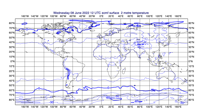
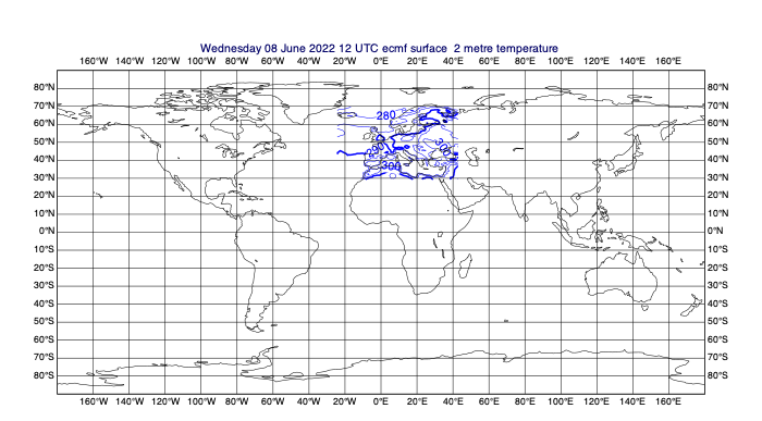
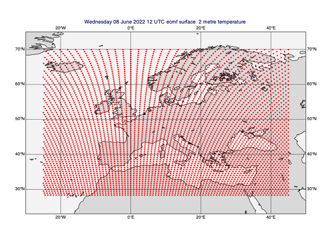
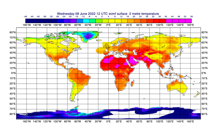
[30]:
# first select 2m temperature and plot it to see what we've got
few_fields = data.select(shortName='2t')
mv.plot(few_fields)
[30]:
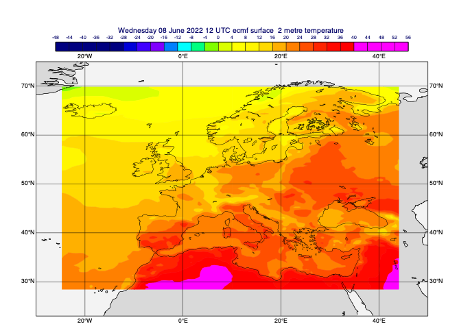
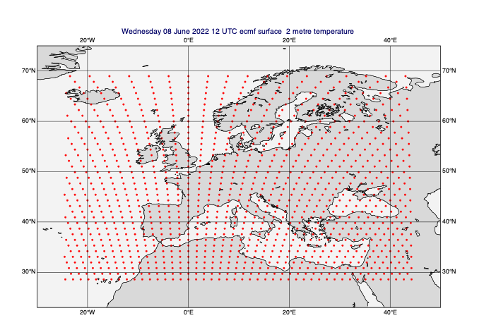
[31]:
# select an area [N,W,S,E]
data_area = [70, -25, 28, 45]
data_on_subarea = mv.read(data=few_fields, area=data_area)
[32]:
# plot the fields to see
mv.plot(data_on_subarea)
[32]:
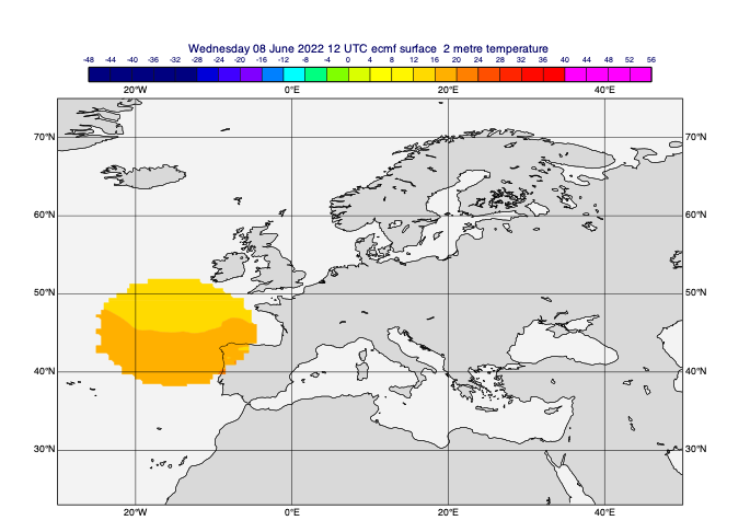
[33]:
# add some automatic styling and zoom into the area
margins = [5, -5, -5, 5]
view_area = [a + b for a, b in zip(data_area, margins)]
coastlines = mv.mcoast(map_coastline_land_shade=True,
                       map_coastline_land_shade_colour="RGB(0.85,0.85,0.85)",
                       map_coastline_sea_shade=True,
                       map_coastline_sea_shade_colour="RGB(0.95,0.95,0.95)",)
view = mv.geoview(map_area_definition="corners", area=view_area, coastlines=coastlines)
cont_auto = mv.mcont(legend=True, contour_automatic_setting="ecmwf", grib_scaling_of_derived_fields=True)
mv.plot(view, data_on_subarea, cont_auto)
[33]:
Point reduction with regridding
[34]:
# let's plot the data points to see what the grid looks like
gridpoint_markers = mv.mcont(
    contour                          = "off",
    contour_grid_value_plot          = "on",
    contour_grid_value_plot_type     = "marker",
    contour_grid_value_marker_height = 0.2,
    contour_grid_value_marker_index  = 15,
    )
mv.plot(view, data_on_subarea[0], gridpoint_markers)
[34]:
[35]:
# regrid to a lower-resolution octahedral reduced Gaussian grid
lowres_data = mv.read(data=data_on_subarea, grid="O80")
mv.plot(view, lowres_data[0], gridpoint_markers)
[35]:
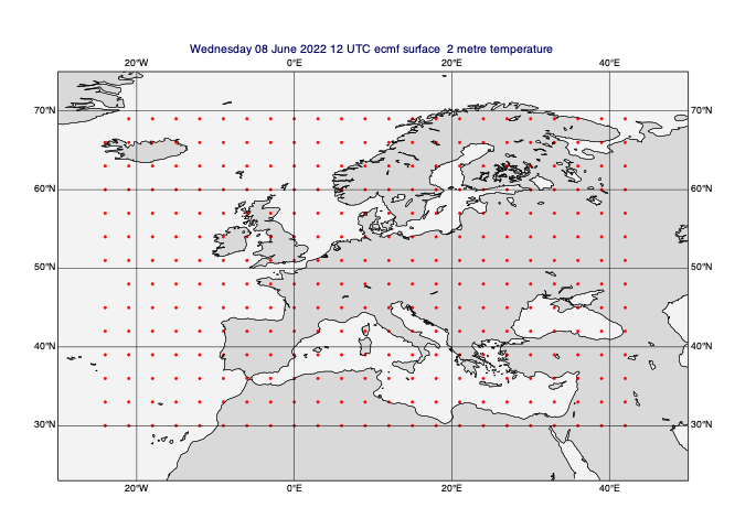
[36]:
# regrid to a regular lat/lon grid
lowres_data = mv.read(data=data_on_subarea, grid=[3, 3]) # 3 degrees
mv.plot(view, lowres_data[0], gridpoint_markers)
[36]:
Masking
[37]:
# masking in Metview means defining an area and either:
#   creating a field with 1s inside the area and 0s outside (missing=False)
#   or
#   turning the values outside the area into missing values (missing=True)
[38]:
# we will use temperature data at step 0 to be masked
t0 = data.select(shortName='2t', step=0)
Geographic masking
This is where we define regions of a field to be preserved, while the points outside those regions are filled with missing values.
[39]:
# define a rectangular mask
rect_masked_data = mv.mask(t0, [48, -12, 63, 5], missing=True) # [N,W,S,E]
mv.plot(view, rect_masked_data, cont_auto)
[39]:
[40]:
# define a circular mask - centre in lat/lon, radius in m
circ_masked_data = mv.rmask(t0, [45, -15, 800*1000], missing=True) # [N,W,S,E]
mv.plot(view, circ_masked_data, cont_auto)
[40]:
[41]:
# polygon area - we will use a shapefile from Magics
import shapefile # pip install pyshp

# download a shapefile with geographic shapes
filename = "ne_50m_land.zip"
if not mv.exist(filename):
    mv.gallery.load_dataset(filename)

sf = shapefile.Reader("ne_50m_land.shp")
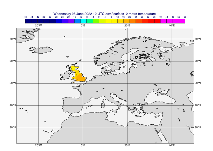
[42]:
# extract the list of points for the Great Britain polygon
shapes = sf.shapes()
points = shapes[135].points  # GB
lats = np.array([p[1] for p in points])
lons = np.array([p[0] for p in points])
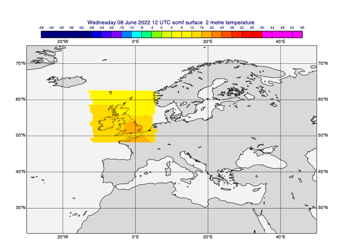
[43]:
poly_masked_data = mv.poly_mask(t0, lats, lons, missing=True)
mv.plot(view, poly_masked_data, cont_auto)
[43]:
Frames
Frames are useful to supply boundary conditions to a local area model.
[44]:
# the frame parameter is the width of the frame in number of grid points
data_frame = mv.read(data=t0, area=data_area, frame=5, grid=[1,1])
mv.plot(data_frame, cont_auto)
[44]:
[45]:
print('mean value for original data    :', t0.average())
print('mean value for rect masked data :', rect_masked_data.average())
print('mean value for circ masked data :', circ_masked_data.average())
print('mean value for poly masked data :', poly_masked_data.average())
print('mean value for framed data      :', data_frame.average())
mean value for original data    : 290.50474329841205
mean value for rect masked data : 286.387063778148
mean value for circ masked data : 289.58698738395395
mean value for poly masked data : 288.6206938091077
mean value for framed data      : 293.29336794339696
Computational masking
This is where we generate masks consisting of 1s where the points are inside a given region (or satisfy some other criteria) and 0s otherwise. We can then combine these and use them to provide a missing value mask to any field.
[46]:
# contouring for 0 and 1 values
mask_1_and_0_contouring = mv.mcont(
    legend="on",
    contour="off",
    contour_level_selection_type="level_list",
    contour_level_list=[0, 1, 2],
    contour_shade="on",
    contour_shade_technique="grid_shading",
    contour_shade_max_level_colour="red",
    contour_shade_min_level_colour="yellow",
)
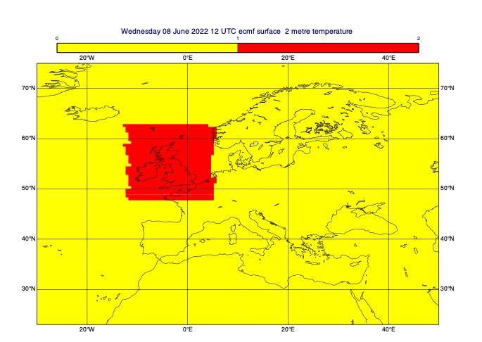
[47]:
# define a rectangular mask
rect_masked_data = mv.mask(t0, [48, -12, 63, 5], missing=False) # [N,W,S,E]
mv.plot(view, rect_masked_data, mask_1_and_0_contouring)
[47]:
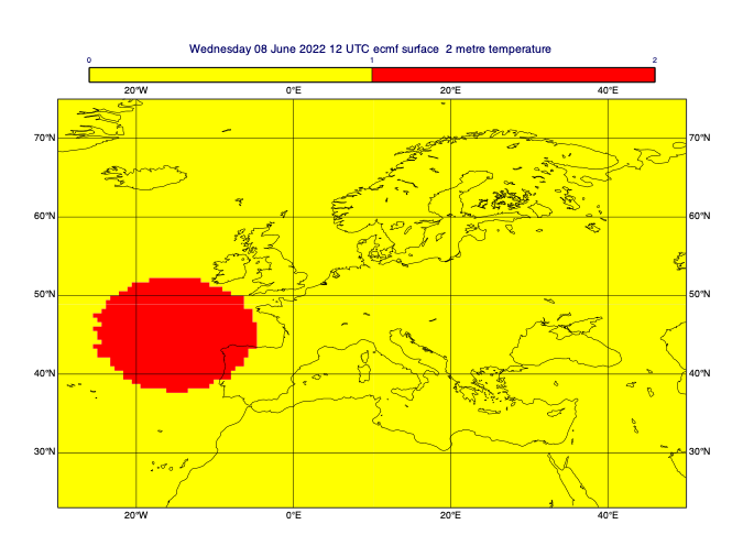
[48]:
# define a circular mask - centre in lat/lon, radius in m
circ_masked_data = mv.rmask(t0, [45, -15, 800*1000], missing=False) # [N,W,S,E]
mv.plot(view, circ_masked_data, mask_1_and_0_contouring)
[48]:
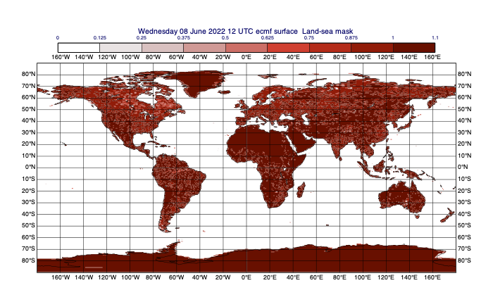
[49]:
# we will now define a mask based on the land-sea mask field; let's plot it first
lsm = data.select(shortName='lsm')
lsm_contour = mv.mcont(
    legend=True,
    contour=False,
    contour_label=False,
    contour_max_level=1.1,
    contour_shade='on',
    contour_shade_technique='grid_shading',
    contour_shade_method='area_fill',
    contour_shade_min_level_colour='white',
    contour_shade_max_level_colour='brown',
)
mv.plot(lsm, lsm_contour)
[49]:
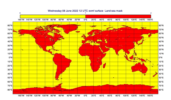
[50]:
# for the purposes of our mask, consider lsm>0.5 to be land
land = lsm > 0.5
mv.plot(land, mask_1_and_0_contouring)
[50]:
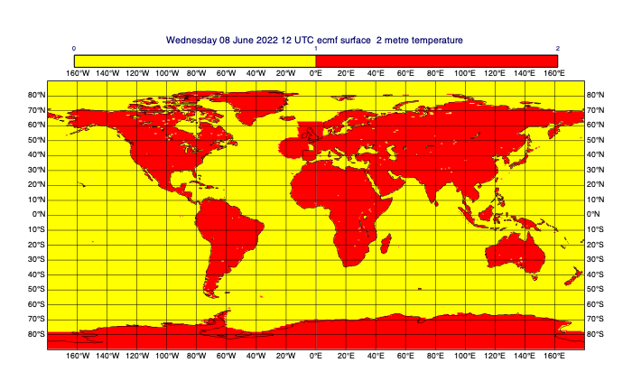
[51]:
# combine the masks with the 'or' operator (only useful for 1/0 masks)
# use '&' to compute the intersection of masks
combined_mask_data = rect_masked_data | circ_masked_data | land
mv.plot(combined_mask_data, mask_1_and_0_contouring)
[51]:
[52]:
# use this mask to replace 0s with missing values in the original data
combined_mask_data = mv.bitmap(combined_mask_data, 0) # replace 0 with missing vals
masked_data = mv.bitmap(t0, combined_mask_data) # copy missing vals over
mv.plot(masked_data, cont_auto)
[52]:
Vertical profiles
Vertical profiles can be extracted from GRIB data for a given point or area (with spatial averaging) for each timestep separately.
[53]:
t0 = data.select(shortName='t', step=0)
t0.ls()
[53]:
| centre | shortName | typeOfLevel | level | dataDate | dataTime | stepRange | dataType | gridType | |
|---|---|---|---|---|---|---|---|---|---|
| Message | |||||||||
| 0 | ecmf | t | isobaricInhPa | 1000 | 20220608 | 1200 | 0 | fc | reduced_gg |
| 1 | ecmf | t | isobaricInhPa | 925 | 20220608 | 1200 | 0 | fc | reduced_gg |
| 2 | ecmf | t | isobaricInhPa | 850 | 20220608 | 1200 | 0 | fc | reduced_gg |
| 3 | ecmf | t | isobaricInhPa | 700 | 20220608 | 1200 | 0 | fc | reduced_gg |
| 4 | ecmf | t | isobaricInhPa | 500 | 20220608 | 1200 | 0 | fc | reduced_gg |
| 5 | ecmf | t | isobaricInhPa | 400 | 20220608 | 1200 | 0 | fc | reduced_gg |
| 6 | ecmf | t | isobaricInhPa | 300 | 20220608 | 1200 | 0 | fc | reduced_gg |
| 7 | ecmf | t | isobaricInhPa | 250 | 20220608 | 1200 | 0 | fc | reduced_gg |
| 8 | ecmf | t | isobaricInhPa | 200 | 20220608 | 1200 | 0 | fc | reduced_gg |
| 9 | ecmf | t | isobaricInhPa | 150 | 20220608 | 1200 | 0 | fc | reduced_gg |
| 10 | ecmf | t | isobaricInhPa | 100 | 20220608 | 1200 | 0 | fc | reduced_gg |
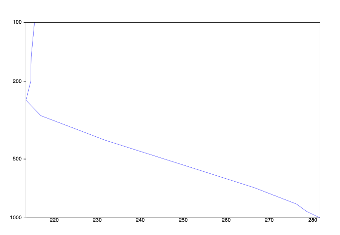
[54]:
# the vertical profile view extracts the data for every level and generates a plot
vpview = mv.mvertprofview(
    input_mode="point",
    point=[-50, -70], # lat,lon
    bottom_level=1000,
    top_level=100,
    vertical_scaling="log",)
mv.plot(vpview, t0)
[54]:
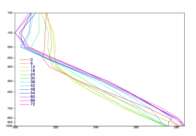
[55]:
# let's plot a profile for each forecast step of temperature

# we will extract one Fieldset for each time step - each of these Fieldsets
# will contain all the vertical levels of temperature data for that time step
# we will end up with a list of these Fieldsets and plot a profile for each

steps = mv.unique(mv.grib_get_long(data, 'step'))
data_for_all_steps = [data.select(shortName='t', step=s) for s in steps]
for f in data_for_all_steps:
    print(f.grib_get_long('step')[0], f.grib_get_long('level'))
0.0 [1000.0, 925.0, 850.0, 700.0, 500.0, 400.0, 300.0, 250.0, 200.0, 150.0, 100.0]
6.0 [1000.0, 925.0, 850.0, 700.0, 500.0, 400.0, 300.0, 250.0, 200.0, 150.0, 100.0]
12.0 [1000.0, 925.0, 850.0, 700.0, 500.0, 400.0, 300.0, 250.0, 200.0, 150.0, 100.0]
18.0 [1000.0, 925.0, 850.0, 700.0, 500.0, 400.0, 300.0, 250.0, 200.0, 150.0, 100.0]
24.0 [1000.0, 925.0, 850.0, 700.0, 500.0, 400.0, 300.0, 250.0, 200.0, 150.0, 100.0]
30.0 [1000.0, 925.0, 850.0, 700.0, 500.0, 400.0, 300.0, 250.0, 200.0, 150.0, 100.0]
36.0 [1000.0, 925.0, 850.0, 700.0, 500.0, 400.0, 300.0, 250.0, 200.0, 150.0, 100.0]
42.0 [1000.0, 925.0, 850.0, 700.0, 500.0, 400.0, 300.0, 250.0, 200.0, 150.0, 100.0]
48.0 [1000.0, 925.0, 850.0, 700.0, 500.0, 400.0, 300.0, 250.0, 200.0, 150.0, 100.0]
54.0 [1000.0, 925.0, 850.0, 700.0, 500.0, 400.0, 300.0, 250.0, 200.0, 150.0, 100.0]
60.0 [1000.0, 925.0, 850.0, 700.0, 500.0, 400.0, 300.0, 250.0, 200.0, 150.0, 100.0]
66.0 [1000.0, 925.0, 850.0, 700.0, 500.0, 400.0, 300.0, 250.0, 200.0, 150.0, 100.0]
72.0 [1000.0, 925.0, 850.0, 700.0, 500.0, 400.0, 300.0, 250.0, 200.0, 150.0, 100.0]
[56]:
# we will plot the profile for each step in a different colour - generate a list
# of 'mgraph' definitions, each using a different colour, for this purpose
nsteps = len(steps)
colour_inc = 1/nsteps
graph_colours = [mv.mgraph(legend=True,
                           graph_line_thickness=2,
                           graph_line_colour='HSL('+str(360*s*colour_inc)+',1,0.45)') for s in range(len(steps))]

# define a nice legend
legend = mv.mlegend(
    legend_display_type="disjoint",
    legend_entry_plot_direction="column",
    legend_text_composition="user_text_only",
    legend_entry_plot_orientation="top_bottom",
    legend_border_colour="black",
    legend_box_mode="positional",
    legend_box_x_position=2.5,
    legend_box_y_position=4,
    legend_box_x_length=5,
    legend_box_y_length=8,
    legend_text_font_size=0.4,
    legend_user_lines=[str(int(s)) for s in steps],
)

# define the axis labels
vertical_axis = mv.maxis(
    axis_type="position_list",
    axis_tick_position_list=data_for_all_steps[0].grib_get_long('level')
)
[57]:
# finally, the magic happens here - the vertical profile view extracts the data
# at the given point at each level
vpview = mv.mvertprofview(
    input_mode="point",
    point=[-50, -70], # lat,lon
    bottom_level=1000,
    top_level=100,
    vertical_scaling="log",
    level_axis=vertical_axis
)
mv.plot(vpview, list(zip(data_for_all_steps, graph_colours)), legend)
[57]:
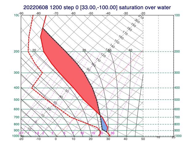
Thermodynamic profiles
A special version of the point profile extraction is implemented by mthermo_grib(), which generates input data for thermodynamic diagrams (e.g. tephigrams). Metview is able to use these profiles to compute thermodynamic parcel paths and stability parameters like CAPE and CIN.
[58]:
# extract temperature and specific humidity for all the levels
# for a given timestep
tq_data = data.select(shortName=["t", "q"], step=0)

# extract thermo profile
location = [33, -100]  # lat, lon
prof = mv.thermo_grib(coordinates=location, data=tq_data)

# compute parcel path - maximum cape up to 700 hPa from the surface
parcel = mv.thermo_parcel_path(prof, {"mode": "most_unstable", "top_p": 700})

# create plot object for parcel areas and path
parcel_area = mv.thermo_parcel_area(parcel)
parcel_vis = mv.xy_curve(parcel["t"], parcel["p"], "charcoal", "dash", 6)

# define temperature and dewpoint profile style
prof_vis = mv.mthermo(
    thermo_temperature_line_thickness=5, thermo_dewpoint_line_thickness=5
)

# define a skew-T thermodynamic diagram view
view = mv.thermoview(type="skewt")

# plot the profile, parcel areas and parcel path together
mv.plot(view, parcel_area, prof, prof_vis, parcel_vis)
[58]:
Vertical cross sections
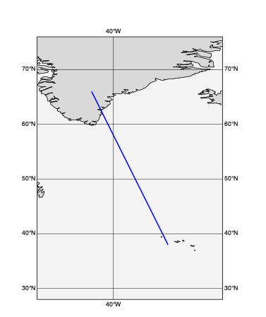
For a vertical cross section data is extracted along a transect line for all the vertical levels for a given timestep. We can choose wether we want to generate the cross section by interpolating the values onto the transect line or use the nearest gridpoint method.
Using the cross section view
The simplest way to generate a cross section is to use the cross section view (mxsectview()), which will automatically preform the data extraction on the input GRIB fields.
[59]:
# define the cross section line
line=[66, -44, 38,-30] # lat1,lon1,lat2,lon2
[87]:
def plot_geo_line(line):
    margins = [10, -10, -10, 10]
    view_area = [a + b for a, b in zip(line, margins)]
    view = mv.geoview(map_area_definition="corners", area=view_area, coastlines=coastlines)
    geoline = mv.mvl_geoline(*line, 0.1)
    mgr = mv.mgraph(graph_line_thickness=3)
    return mv.plot(view, geoline, mgr)

plot_geo_line(line)
[87]:
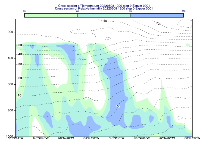
[61]:
# define the cross section view
cs_view = mv.mxsectview(
    bottom_level=1000,
    top_level=100,
    line=line,
    horizontal_point_mode="interpolate",
)

# extract temperature and relative humidity for the first timestep
# for all the levels. We scale temperature values from to Celsius units
# for plotting
t = data.select(shortName="t", step=0) - 273.16
r = data.select(shortName="r", step=0)

# define the contouring styles for the cross section
cont_xs_t = mv.mcont(
    contour_line_style           = "dash",
    contour_line_colour          = "black",
    contour_highlight            = "off",
    contour_level_selection_type = "interval",
    contour_interval             = 5
    )

cont_xs_r = mv.mcont(
    contour_automatic_setting = "style_name",
    contour_style_name        = "sh_grnblu_f65t100i15_light",
    legend                    = "on"
    )

# generate the cross section plot. The computations are automatically performed according
# to the settings in the view.
mv.plot(cs_view, r, cont_xs_r, t, cont_xs_t)
[61]:
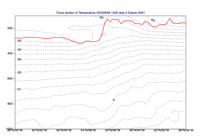
Accessing the cross section data
The actual results of the cross section computations are stored in a custom NetCDF format. If we want to access it mcross_sect() should be used instead of the view.
[62]:
# compute cross section data for temperature
xs_t = mv.mcross_sect(
    data=t,
    bottom_level=1000,
    top_level=100,
    line=line,
    horizontal_point_mode="interpolate")

# write netCDF  data to disk
mv.write("xs_t.nc", xs_t)

# dump the data contents
import xarray as xr
ds_t= xr.open_dataset("xs_t.nc")
ds_t
[62]:
<xarray.Dataset>
Dimensions:  (time: 1, lat: 64, lon: 64, nlev: 11)
Coordinates:
  * time     (time) datetime64[ns] 2022-06-08T12:00:00
  * lat      (lat) float64 66.0 65.56 65.11 64.67 ... 39.33 38.89 38.44 38.0
  * lon      (lon) float64 -44.0 -43.78 -43.56 -43.33 ... -30.44 -30.22 -30.0
Dimensions without coordinates: nlev
Data variables:
    t_lev    (time, nlev) float64 100.0 150.0 200.0 250.0 ... 850.0 925.0 1e+03
    t        (time, nlev, lon) float64 -48.13 -48.13 -48.13 ... 17.39 17.15 17.2
Attributes:
    _FillValue:          1e+22
    _View:               MXSECTIONVIEW
    type:                MXSECTION
    xsHorizontalMethod:  interpolate
title: Cross section of Temperature 20220608 1200 step 0 Ex...Plotting the cross section data and using it for single level slicing
[63]:
# read tropopause pressure (it is a single level field)
trpp = data.select(shortName="trpp", step=0)

# using the temperature cross section object we can extract a slice from trpp along the
# transect line and build a curve object out of it. The pressure has to be scaled
# from Pa to hPa.
trpp_curve = mv.xs_build_curve(xs_t, trpp/100, "red", "solid", 3)

# directly plot the temperature cross section data and the trpp curve
mv.plot(xs_t, cont_xs_t,  trpp_curve)
[63]:
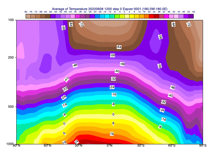
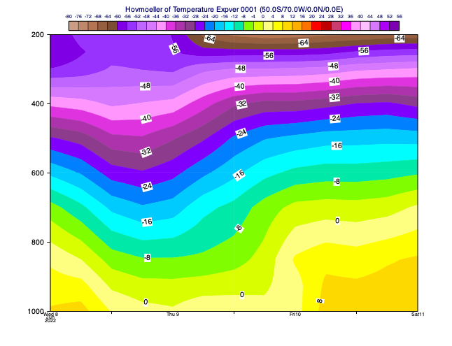
Average vertical cross sections
This is a variant of the vertical cross section where either a zonal or meridional average is computed for all the levels in a given timestep. Similarly to the cross section the input data can be directly plotted into a view (maverageview()) or passed on to mxs_average() to generate average cross section NetCDF data.
[64]:
# set up the average view for a global zonal mean
av_view = mv.maverageview(
    top_level=100,
    bottom_level=1000,
    vertical_scaling="log",
    area=[90,-180, -90, 180], # N, W, S, E
    direction="ew"
)

# extract temperature for the first timestep for all the levels. We scale
# temperature values to Celsius units for plotting
t = data.select(shortName="t", step=0)
t = t - 273.16

# define the contouring styles for the zonal mean cross section
cont_zonal_t = mv.mcont(
    contour_automatic_setting = "style_name",
    contour_style_name        = "sh_all_fM80t56i4_v2",
    legend                    = "on"
    )

# generate the average cross section plot. The computations are automatically
# performed according to the settings in the view.
mv.plot(av_view, t, cont_zonal_t)
[64]:
Hovmoeller diagrams
Hovmoeller diagrams are special sections for (mostly single level) fields where one axis is always the time while the other one can be derived in various ways. Metview supports 3 flavours of it: - area Hovmoellers - vertical Hovmoellers - line Hovmoellers
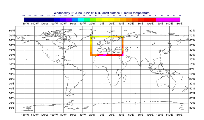
Area Hovmoeller diagrams
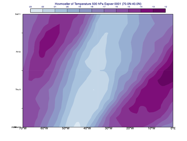
In this diagram type for each date and time either zonal or meridional averaging is performed on the data. The example below shows a Hovmoeller diagram with longitude on the horizontal axis and time on the vertical axis. Each point in the plot is a meridional average performed for temerature on 500 hPa at the given time in North-South (meridional) direction.
[65]:
# define the Hovmoeller view for an area in the North-Atlantic and
# choose meridional averaging
view = mv.mhovmoellerview(
    type="area_hovm",
    area=[70, -70, 40, 0],
    average_direction="north_south",
)

# extract temperature on 500 hPa for all the timestep and
# convert it into Celsius units for plotting
t = data.select(shortName="t", level=500)
t = t - 273.16

# define contour shading
cont_hov_t = mv.mcont(
    legend                       = "on",
    contour                      = "off",
    contour_level_selection_type = "interval",
    contour_max_level            = -12,
    contour_min_level            = -23,
    contour_interval             = 1,
    contour_label                = "off",
    contour_shade                = "on",
    contour_shade_colour_method  = "palette",
    contour_shade_method         = "area_fill",
    contour_shade_palette_name   = "m_purple2_11"
    )

# generate the area Hovmoeller plot. The computations are automatically
# performed according to the settings in the view.
mv.plot(view, t, cont_hov_t)
[65]:
Vertical Hovmoeller diagrams
In this diagram type the horizontal axis is time and the vertical axis is a vertical co-ordinate. The data is extracted for a given location or generated by spatial averaging over an area. The example below shows the temperature forecast evolution for a selected point having pressure as the vertical axis.
[66]:
# define a vertical Hovmoeller view for a location. The point data
# is extracted with the nearest gridpoint method
view = mv.mhovmoellerview(
    type="vertical_hovm",
    bottom_level=1000,
    top_level=200,
    input_mode="nearest_gridpoint",
    point=[-50, -70],
)

# extract the temperature on all the levels and timesteps. Values
# scaled to Celsius units for plotting
t = data.select(shortName="t")
t = t - 273.16

# generate the vertical Hovmoeller plot. The computations are automatically
# performed according to the settings in the view.
mv.plot(view, t, cont_zonal_t)
[66]:
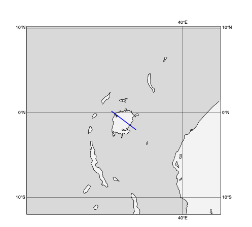
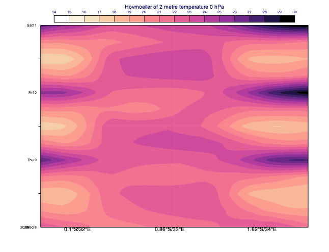
Line Hovmoeller diagrams
In this diagram type the data is extracted along a transect line from a single level field for multiple dates and times. In the resulting plot one axis is time while the other goes along the transect line. The example below shows a line Hovmoeller diagram for the 2m temperature forecast evolution along a line across Lake Victoria.
[88]:
# define a line Hovmoeller view for a transect line across Lake Victoria
line_across_lake_victoria = [0.2, 31.6, -2, 34.5]  # N,W,S,E
plot_geo_line(line_across_lake_victoria)
[88]:
[68]:
hov_view = mv.mhovmoellerview(
    type="line_hovm",
    line=line_across_lake_victoria,
    resolution=0.25,
    swap_axis="no"
)

# extract the 2m temperature on all the levels and timesteps. Values
# scaled to Celsius units for plotting
t = data.select(shortName="2t")
t = t -273.16

# define contour shading for t2m
t_cont = mv.mcont(
    legend="on",
    contour="off",
    contour_level_selection_type="interval",
    contour_max_level=30,
    contour_min_level=14,
    contour_interval=1,
    contour_label="off",
    contour_shade="on",
    contour_shade_colour_method="palette",
    contour_shade_method="area_fill",
    contour_shade_palette_name="m_orange_purple_16",
)

# generate the line Hovmoeller plot. The computations are automatically
# performed according to the settings in the view.
mv.plot(hov_view, t, t_cont)
[68]:
Gridpoint selection
[69]:
# get value of single field at location
r1000 = data['r1000']
bologna_coords = [44.5, 11.3]
[70]:
print(r1000.nearest_gridpoint(bologna_coords))
46.73977756500244
[71]:
# get more info about the point
print(r1000.nearest_gridpoint_info(bologna_coords))
[{'latitude': 44.6489, 'longitude': 11.6471, 'index': 14251.0, 'distance': 32.0703, 'value': 46.7398}]
[72]:
# get value of multiple fields at a single location
r = data['r']
print(r.nearest_gridpoint(bologna_coords))
[46.73977756500244, 63.34179496765137, 62.7387580871582, 54.288533210754395, 32.877156257629395, 34.60153579711914, 82.47459983825684, 101.11736679077148, 42.8692102432251, 3.479970932006836, 2.4789832830429077]
[73]:
# get value of single field at multiple locations
lats = np.array([10, 20, 30, 40])
lons = np.array([45, 40, 35, 30])
print(r1000.nearest_gridpoint(lats, lons))
[21.67727757 76.52102757 18.95852757 56.11477757]
[74]:
# get value of multiple fields at multiple locations (returns 2d numpy array)
lats = np.array([10, 20, 30, 40])
lons = np.array([45, 40, 35, 30])
print(r.nearest_gridpoint(lats, lons))
[[21.67727757 76.52102757 18.95852757 56.11477757]
 [24.24804497 20.84179497 20.74804497 60.49804497]
 [29.02000809 11.14500809 30.20750809 80.39500809]
 [63.72603321 13.63228321 13.25728321 75.38228321]
 [58.50215626  3.00215626 35.37715626 23.87715626]
 [12.1640358   8.1640358  40.5390358  33.4765358 ]
 [12.41209984  8.72459984 18.16209984 35.53709984]
 [21.36736679 22.24236679 10.11736679 25.05486679]
 [36.86921024 62.77546024 11.24421024  3.33796024]
 [91.01122093 54.79247093 18.57372093  2.72997093]
 [65.22898328 46.91648328 39.57273328  3.94773328]]
[75]:
# interpolate the value at the point (because it does not fall exactly on a grid point)
print(r.interpolate(bologna_coords))
[45.3462287863336, 57.24063741008365, 62.874751901836966, 59.515108579518085, 38.87074203846925, 50.79850151897796, 95.72173420260529, 99.40602160846703, 42.18095344810713, 3.4901434575907517, 2.3958725332532467]
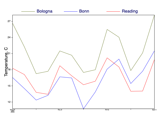
Time series
[76]:
# define the lat/lon coordinates of three locations
bologna_coords = [44.5, 11.3]
bonn_coords    = [50.7, 7.1]
reading_coords = [51.4, 0.98]
[77]:
# extract point data from these locations from the 2m temperature data
t2m = data['2t'] - 273.16

bologna_vals = t2m.nearest_gridpoint(bologna_coords)
bonn_vals = t2m.nearest_gridpoint(bonn_coords)
reading_vals = t2m.nearest_gridpoint(reading_coords)
print(reading_vals)

# extract the valid times for the data
times = mv.valid_date(t2m)
times
[18.27154541015625, 17.10321044921875, 13.79827880859375, 13.430252075195312, 18.741119384765625, 16.882583618164062, 15.208755493164062, 15.868255615234375, 20.207778930664062, 18.510986328125, 13.99456787109375, 14.033859252929688, 19.8885498046875]
[77]:
[datetime.datetime(2022, 6, 8, 12, 0),
 datetime.datetime(2022, 6, 8, 18, 0),
 datetime.datetime(2022, 6, 9, 0, 0),
 datetime.datetime(2022, 6, 9, 6, 0),
 datetime.datetime(2022, 6, 9, 12, 0),
 datetime.datetime(2022, 6, 9, 18, 0),
 datetime.datetime(2022, 6, 10, 0, 0),
 datetime.datetime(2022, 6, 10, 6, 0),
 datetime.datetime(2022, 6, 10, 12, 0),
 datetime.datetime(2022, 6, 10, 18, 0),
 datetime.datetime(2022, 6, 11, 0, 0),
 datetime.datetime(2022, 6, 11, 6, 0),
 datetime.datetime(2022, 6, 11, 12, 0)]
[78]:
vaxis = mv.maxis(axis_title_text="Temperature, C", axis_title_height=0.5)

ts_view = mv.cartesianview(
    x_automatic="on",
    x_axis_type="date",
    y_automatic="on",
    vertical_axis=vaxis,
)

# create the curves for all locations
curve_bologna = mv.input_visualiser(
    input_x_type="date", input_date_x_values=times, input_y_values=bologna_vals
)

curve_bonn = mv.input_visualiser(
    input_x_type="date", input_date_x_values=times, input_y_values=bonn_vals
)

curve_reading = mv.input_visualiser(
    input_x_type="date", input_date_x_values=times, input_y_values=reading_vals
)

# set up visual styling for each curve
common_graph = {"graph_line_thickness": 2, "legend": "on"}
graph_bologna = mv.mgraph(common_graph, graph_line_colour="olive", legend_user_text="Bologna")
graph_bonn = mv.mgraph(common_graph, graph_line_colour="blue", legend_user_text="Bonn")
graph_reading = mv.mgraph(common_graph, graph_line_colour="red", legend_user_text="Reading")

# customise the legend
legend = mv.mlegend(legend_display_type="disjoint", legend_text_font_size=0.5)

# plot everything into the Cartesian view
mv.plot(ts_view, curve_bologna, graph_bologna, curve_bonn, graph_bonn, curve_reading, graph_reading, legend)
[78]: