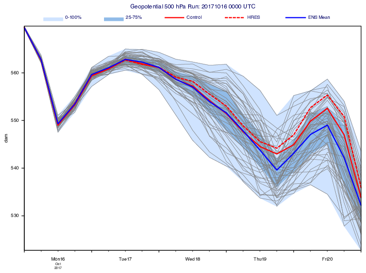
GRIB - ENS Plume

# (C) Copyright 2017- ECMWF.
#
# This software is licensed under the terms of the Apache Licence Version 2.0
# which can be obtained at http://www.apache.org/licenses/LICENSE-2.0.
#
# In applying this licence, ECMWF does not waive the privileges and immunities
# granted to it by virtue of its status as an intergovernmental organisation
# nor does it submit to any jurisdiction.
#

import metview as mv
import numpy as np

# getting data
use_mars = False

# getting forecast data from MARS
if use_mars:
    ret_core = {
        "date": 20171016,
        "time": 0,
        "param": "z",
        "step": list(range(0, 126, 6)),
        "levtype": "pl",
        "levelist": 500,
        "grid": [0.5, 0.5],
        "area": [45, -10, 55, 5],
    }

    # perturbed ENS members
    pf = mv.retrieve(stream="enfo", type="pf", number=["1", "TO", "50"], **ret_core)

    # control member
    cf = mv.retrieve(stream="enfo", type="cf", **ret_core)

    # high-res deterministic
    hr = mv.retrieve(type="fc", **ret_core)

    g = mv.merge(pf, cf, hr)
# read data from file
else:
    filename = "ens_plume.grib"
    if mv.exist(filename):
        g = mv.read(filename)
    else:
        g = mv.gallery.load_dataset(filename)

# define location
location = [52, -7]

# the ensemble size (perturbed members)
ens_num = 50

# extract time series for the pertubations (as a 2D ndarray)
pert = []
for i in range(1, ens_num + 1):
    gf = mv.read(data=g, number=i, type="pf")
    pert.append(mv.nearest_gridpoint(gf, location))
d_pert = np.array(pert)

# extract time series for the control forecast (as 1D array)
gf = mv.read(data=g, type="cf")
d_control = np.array(mv.nearest_gridpoint(gf, location))

# extract time series for the hres deterministic forecast (as a 1D ndarray)
gf = mv.read(data=g, type="fc")
d_hres = np.array(mv.nearest_gridpoint(gf, location))

# convert data to dam units
d_pert = d_pert / (9.81 * 10)
d_control = d_control / (9.81 * 10)
d_hres = d_hres / (9.81 * 10)

# compute ENS mean series
d_mean = np.vstack([d_pert, d_control]).mean(axis=0)

# get metadata for the title
meta = mv.grib_get(gf[0], ["name", "level", "date", "time"])[0]

# get the valid times for the time series points
d_times = mv.valid_date(gf)

# determine number of timesteps
ts_num = len(d_times)

# compute shaded areas (polygons)
# outer area = full ENS range
# inner area = 25-75 percentile range
poly_ts = [None] * (ts_num * 2)
poly_outer = np.empty(ts_num * 2)
poly_inner = np.empty(ts_num * 2)

for i in range(ts_num):
    # collect data (pf+cf) for the given ts
    idx_start = i * ens_num
    idx_end = (i + 1) * ens_num - 1
    v = d_pert[:, i]
    v = np.append(v, d_control[i])

    i_top = i
    i_bottom = 2 * ts_num - i - 1

    poly_ts[i_top] = d_times[i]
    poly_ts[i_bottom] = d_times[i]
    poly_outer[i_top] = mv.maxvalue(v)
    poly_outer[i_bottom] = mv.minvalue(v)
    perc = mv.percentile(v, [25, 75])
    poly_inner[i_top] = perc[1]
    poly_inner[i_bottom] = perc[0]

# define colours for the curves
col_pert = "RGB(0.5,0.5,0.5)"
col_control = "RED"
col_hres = col_control
col_mean = "BLUE"

# define colours for shaded areas
col_outer = "RGB(0.8118,0.8902,1)"
col_inner = "RGB(0.5631,0.7315,0.9114)"

# generate curves for the perturbations
gr_lst = []
for i in range(50):
    gr_lst.append(
        mv.input_visualiser(
            input_x_type="date", input_date_x_values=d_times, input_y_values=d_pert[i]
        )
    )
    gr_lst.append(
        mv.mgraph(graph_line_thickness=1, graph_line_colour=col_pert, legend="off")
    )


# generate curve for the control forecats
gr_lst.append(
    mv.input_visualiser(
        input_x_type="date", input_date_x_values=d_times, input_y_values=d_control
    )
)
gr_lst.append(
    mv.mgraph(
        graph_line_thickness=4,
        graph_line_colour=col_control,
        legend="on",
        legend_user_text="Control",
    )
)

# generate curve for the hres forecast
gr_lst.append(
    mv.input_visualiser(
        input_x_type="date", input_date_x_values=d_times, input_y_values=d_hres
    )
)
gr_lst.append(
    mv.mgraph(
        graph_line_thickness=4,
        graph_line_colour=col_hres,
        graph_line_style="dash",
        legend="on",
        legend_user_text="HRES",
    )
)

# generate curve for the ENS mean
gr_lst.append(
    mv.input_visualiser(
        input_x_type="date", input_date_x_values=d_times, input_y_values=d_mean
    )
)
gr_lst.append(
    mv.mgraph(
        graph_line_thickness=4,
        graph_line_colour=col_mean,
        legend="on",
        legend_user_text="ENS Mean",
    )
)

# generate graphic objects (areas) for the shaded areas
gr_shade_lst = [
    mv.input_visualiser(
        input_x_type="date", input_date_x_values=poly_ts, input_y_values=poly_outer
    ),
    mv.mgraph(
        graph_type="area",
        graph_line_colour=col_outer,
        graph_shade_colour=col_outer,
        legend="on",
        legend_user_text="0-100%",
    ),
    mv.input_visualiser(
        input_x_type="date", input_date_x_values=poly_ts, input_y_values=poly_inner
    ),
    mv.mgraph(
        graph_type="area",
        graph_line_colour=col_inner,
        graph_shade_colour=col_inner,
        legend="on",
        legend_user_text="25-75%",
    ),
]

# set up the Cartesian view to plot into
# including customised axes so that we can change the size
# of the labels and add titles
haxis = mv.maxis(
    axis_type="date",
    axis_tick_size=0.4,
    axis_date_type="days",
    axis_years_label_height=0.3,
    axis_months_label_height=0.3,
    axis_days_label_height=0.4,
    axis_hours_label="on",
    axis_hours_label_colour="white",
    axis_hours_label_height=0.3,
    axis_tip_title="on",
    axis_minor_tick="on",
    axis_minor_tick_count=4,
)

vaxis = mv.maxis(
    axis_title_text="dam", axis_title_height=0.4, axis_tick_label_height=0.4
)

view = mv.cartesianview(
    x_automatic="on",
    x_axis_type="date",
    y_automatic="on",
    horizontal_axis=haxis,
    vertical_axis=vaxis,
)

# define legend
legend = mv.mlegend(legend_display_type="disjoint", legend_text_font_size=0.4)

# define title
title = mv.mtext(
    text_lines=f"{meta[0]} {meta[1]} hPa Run: {meta[2]} {meta[3]} UTC",
    text_font_size=0.5,
)

# define the output plot file
mv.setoutput(mv.pdf_output(output_name="ens_plume"))

# plot everything into the Cartesian view
mv.plot(view, gr_shade_lst, gr_lst, legend, title)