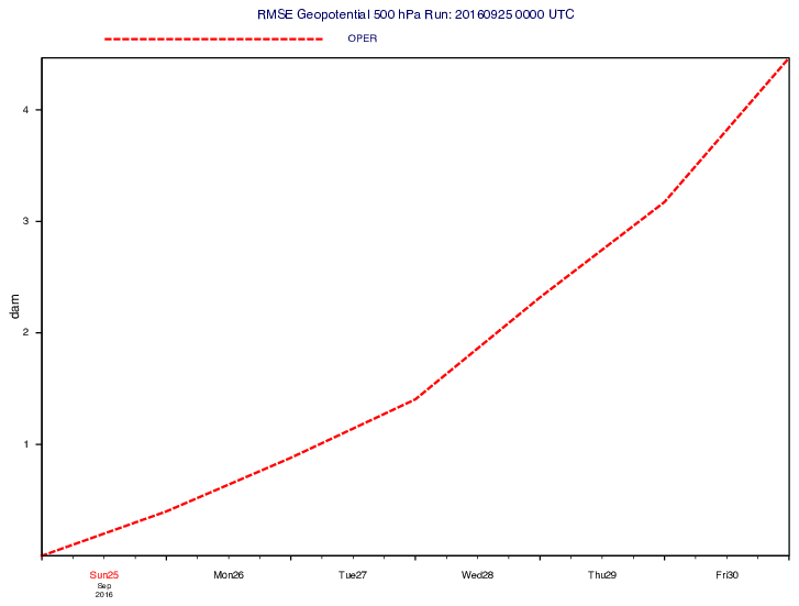
GRIB - RMSE Curve

# (C) Copyright 2017- ECMWF.
#
# This software is licensed under the terms of the Apache Licence Version 2.0
# which can be obtained at http://www.apache.org/licenses/LICENSE-2.0.
#
# In applying this licence, ECMWF does not waive the privileges and immunities
# granted to it by virtue of its status as an intergovernmental organisation
# nor does it submit to any jurisdiction.
#

import metview as mv
import numpy as np

# getting data
use_mars = False

# getting data from MARS
if use_mars:
    steps = list(range(0, 168, 24))
    area = [15, -70, 80, 40]
    grid = [1, 1]
    # analysis
    f1 = mv.retrieve(
        type="an",
        levelist=500,
        date=mv.valid_date(base=mv.date(20160925), step=steps),
        time=0,
        area=area,
        grid=grid,
    )
    # forecast
    f2 = mv.retrieve(
        type="fc",
        levelist=500,
        date=20160925,
        time=0,
        step=steps,
        area=area,
        grid=grid,
    )

    f = mv.merge(f1, f2)

# read data from file
else:
    filename = "z_rmse.grib"
    if mv.exist(filename):
        f = mv.read(filename)
    else:
        f = mv.gallery.load_dataset(filename)

# the input data contains 500 hPa geopotential fields.
# The data is correctly sorted so the an fc fields are
# properly paired up regarding their valid date/time
f_an = mv.read(data=f, type="an")
f_fc = mv.read(data=f, type="fc")

# compute the rmse values
d_fc = mv.sqrt(mv.integrate((f_fc - f_an) ** 2))

# scale the results to dam units
d_fc = np.array(d_fc) / (9.81 * 10)

# get metadata for the title
meta = mv.grib_get(f_fc[0], ["name", "level", "date", "time"])[0]

# get the valid times for the time series points
d_times = mv.valid_date(f_fc)

# generate curve for the forecast
gr_lst = []
gr_lst.append(
    mv.input_visualiser(
        input_x_type="date", input_date_x_values=d_times, input_y_values=d_fc
    )
)
gr_lst.append(
    mv.mgraph(
        graph_line_thickness=4,
        graph_line_colour="red",
        graph_line_style="dash",
        legend="on",
        legend_user_text="OPER",
    )
)

# set up the Cartesian view to plot into
# including customised axes so that we can change the size
# of the labels and add titles
haxis = mv.maxis(
    axis_type="date",
    axis_tick_size=0.4,
    axis_date_type="days",
    axis_years_label_height=0.3,
    axis_months_label_height=0.3,
    axis_days_label_height=0.4,
    axis_hours_label="on",
    axis_hours_label_colour="white",
    axis_hours_label_height=0.3,
    axis_tip_title="on",
    axis_minor_tick="on",
    axis_minor_tick_count=4,
)

vaxis = mv.maxis(
    axis_title_text="dam", axis_title_height=0.5, axis_tick_label_height=0.4
)

view = mv.cartesianview(
    x_automatic="on",
    x_axis_type="date",
    y_automatic="on",
    horizontal_axis=haxis,
    vertical_axis=vaxis,
)

# define legend
legend = mv.mlegend(legend_display_type="disjoint", legend_text_font_size=0.4)

# define title
title = mv.mtext(
    text_lines=f"RMSE {meta[0]} {meta[1]} hPa Run: {meta[2]} {meta[3]} UTC",
    text_font_size=0.5,
)

# define the output plot file3
mv.setoutput(mv.pdf_output(output_name="rmse_curve"))

# plot everything into the Cartesian view
mv.plot(view, gr_lst, legend, title)