Part 2 - GRIB

Note

In Metview GRIB data is represented as a Fieldset.

Setup

Navigate into the 2_grib folder within Metview.

Customising the plot to bring out information

Right-click on the Metview desktop, Create new icon and select Contouring. Rename the newly created icon to ‘shade’ and edit it, setting these parameters:

Parameter	Value
Legend	On
Contour Shade	On
Contour Shade Method	Area Fill

You can also play with the colour settings. When done, click OK to close the editor, then visualise the GRIB file and drop your shade icon into the plot window. There are loads of options in the Contouring icon, which exposes all of the Magics parameters. Supplied in the folder are some additional Contouring icons for you to try dropping into the plot window to see what effect they have.

Icon	Description
shade30	30 contour levels, no isolines
grid_shade	no interpolation, just shade the grid boxes (looks best with anti-aliasing turned off)
marker_shade	plots a coloured marker at each grid point location (best for categorical data)
grid_points	plots a small marker at each grid point location (all markers are the same, not dependent on value ; good for seeing grid structure)
grid_vals	plots values at each grid point location (zoom into a small area before applying this ; good for inspecting values ; drop the land_sea_shade icon into the plot window too to get better orientation)

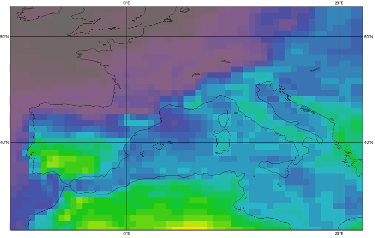
Have a look at the supplied Python script plot_max_value_locations.py and execute it. It shows one way to plot the locations of the highest values, by masking off the lower values as invalid. Another way would be a customised Contouring icon that only plotted large values.

Examine the GRIB metadata

Right-click on the GRIB file icon and choose Examine. This brings up the GRIB examiner tool - have a look!

If you find this tool useful, you can invoke it directly from the command line:

metview -e grib <path/to/grib/file>

If you have time…

Compute and plot a time series from a point

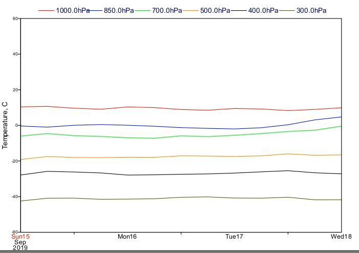
Look at the supplied script plot_time_series.py as an example. It takes a GRIB file containing temperature data on multiple vertical levels for multiple time steps. The script plots a time series for each level for a given grid point.

Convert a GRIB field into text format

Create a new Grib to Geopoints icon. Edit it and drop one of the GRIB files into the Data box as shown.

Executing this icon will convert the first GRIB field into Geopoints format. The result can be directly visualised, examined or saved to disk.

Get a Python xarray from a GRIB file

The script grib_xarray.py shows how to get an xarray from a GRIB file. See the Computing ensemble mean and spread with xarray and plotting the results with Metview Jupyter notebook for a more detailed example using ensemble data.