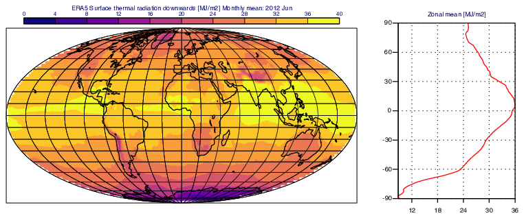
GRIB - Map with Zonal Mean Curve

# (C) Copyright 2017- ECMWF.
#
# This software is licensed under the terms of the Apache Licence Version 2.0
# which can be obtained at http://www.apache.org/licenses/LICENSE-2.0.
#
# In applying this licence, ECMWF does not waive the privileges and immunities
# granted to it by virtue of its status as an intergovernmental organisation
# nor does it submit to any jurisdiction.
#

import metview as mv
import numpy as np

# getting data
use_cds = False

filename = "strd_era5.grib"

# getting data from CDS
if use_cds:
    import cdsapi

    c = cdsapi.Client()
    c.retrieve(
        "reanalysis-era5-single-levels-monthly-means",
        {
            "format": "grib",
            "variable": "surface_thermal_radiation_downwards",
            "year": "2012",
            "month": "06",
            "time": "00:00",
            "product_type": "monthly_averaged_reanalysis",
        },
        filename,
    )

    g = mv.read(filename)
# read data from file
else:
    if mv.exist(filename):
        g = mv.read(filename)
    else:
        g = mv.gallery.load_dataset(filename)

# scale data values from J/m2 to MJ/m2
g = g * 1e-6

# compute zonal mean with a 1 degree bin
m = mv.average_ew(g, [90, -180, -90, 180], 1)
m_lat = np.linspace(90, -90, 181)

# generate zonal mean curve data
c = mv.xy_curve(m, m_lat, "red", "solid", 2)

# define view for map
coastlines = mv.mcoast(map_coastline_thickness=2, map_label="off")

map_view = mv.geoview(map_projection="mollweide", coastlines=coastlines)

# define curve view
horizontal_axis = mv.maxis(
    axis_orientation="horizontal",
    axis_tick_label_height=0.4,
    axis_grid="on",
    axis_grid_line_style="dot",
)

vertical_axis = mv.maxis(
    axis_orientation="verical",
    axis_tick_label_height=0.4,
    axis_grid="on",
    axis_grid_line_style="dot",
)

curve_view = mv.cartesianview(
    x_automatic="on",
    y_automatic="off",
    y_min=-90,
    y_max=90,
    horizontal_axis=horizontal_axis,
    vertical_axis=vertical_axis,
)

# build layout (20cm x 8 cm)
page_0 = mv.plot_page(right=75, view=map_view)

page_1 = mv.plot_page(left=75, view=curve_view)

dw = mv.plot_superpage(
    pages=[page_0, page_1],
    layout_size="custom",
    custom_width=20,
    custom_height=8,
)

# define contour shading
cont_shade = mv.mcont(
    legend="on",
    contour="off",
    contour_level_selection_type="interval",
    contour_max_level=40,
    contour_min_level=0,
    contour_interval=4,
    contour_label="off",
    contour_shade="on",
    contour_shade_colour_method="palette",
    contour_shade_method="area_fill",
    contour_shade_palette_name="matplotlib_Plasma_10",
)

# define legend
legend = mv.mlegend(legend_text_font_size=0.35)

# define titles
title_map = mv.mtext(
    text_lines="ERA5 <grib_info key='name'/> [MJ/m2] Monthly mean: <grib_info key='valid-date' format='%Y %b'/>",
    text_font_size=0.4,
)

title_curve = mv.mtext(text_lines="Zonal mean [MJ/m2]", text_font_size=0.4)

# define the output plot file
mv.setoutput(mv.pdf_output(output_name="map_and_zonal_mean_curve"))

# generate plot
mv.plot(dw[0], g, cont_shade, legend, title_map, dw[1], c, title_curve)