Part 4 - ODB

Note

ODB data is represented by an Odb object in Metview.

Setup

Navigate into the 4_odb/main folder within Metview.

Retrieving ODB data from MARS

Use the ‘ret_temp’ Mars Retrieval icon to fetch Land TEMP ODB data from MARS for a given date. Edit the icon (right-click & edit) to see what parameters are set. The most important ones are as follows:

Parameter	Value	Description
Type	MFB	Mondb feedback
Obsgroup	17	Conventional
Reportype	16022	Land TEMP

Close the icon editor and perform the data retrieval by choosing execute from the icon’s context menu. The icon name should turn orange whilst the retrieval takes place, then green to indicate success.

Note

If ‘ret_temp’ does not turn green after half a minute probably there is a problem with MARS. In this case find the ‘backup.temp.odb’ ODB Database icon at the top-right of the folder and rename it ‘temp.odb’ (right-click and rename). This icon contains the very same data that we wanted to retrieve from MARS.

If the MARS retrieval was successful the data is now cached locally. To save the ODB data from the cache to disk, right-click Save result on the Mars Retrieval icon and save as ‘temp.odb’. A few seconds later an ODB Database icon with the given name will appear at the bottom of your folder.

Examine the ODB file

To see what was retrieved, right-click examine the icon. This brings up Metview’s ODB Examiner tool.

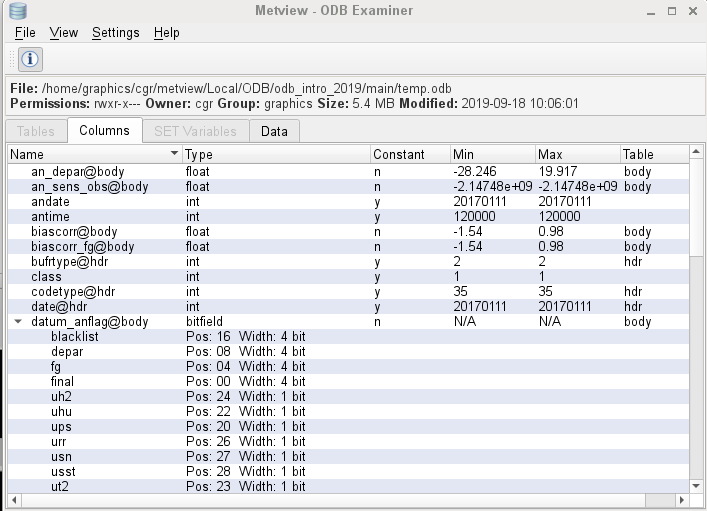
Here you can see the metadata (Columns tab) and the actual data values themselves as well (Data tab). Close the ODB Examiner.

Interactive Visualisation

Using the ODB Visualiser

We will visualise the 500 hPa temperature values from our ODB by editing the supplied ‘vis_temp’ ODB Visualiser icon. The ODB/SQL query we need to perform is as follows:

select
  lat@hdr,
  lon@hd,
  obsvalue@body
where
  varno = 2 and vertco_reference_1=50000

Now edit the ‘vis_temp’ icon and set the following parameters:

Odb Data	Drop the temp.odb icon into this box
Odb Where	varno = 2 and vertco_reference_1=50000

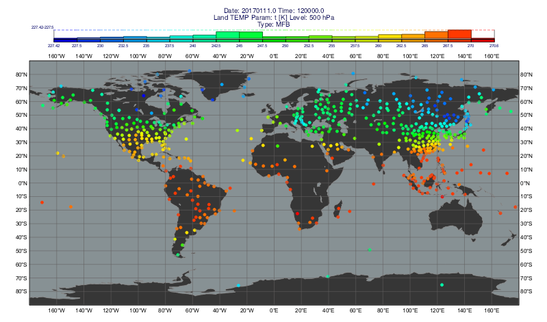
Save the icon and visualise it. Then drag the the provided Symbol Plotting, Coastlines, Legend and Text Plotting icons into the plot for further customisation (either one at a time, or all together). Keep the plot window open.

Inspecting the Data Values in the Plot

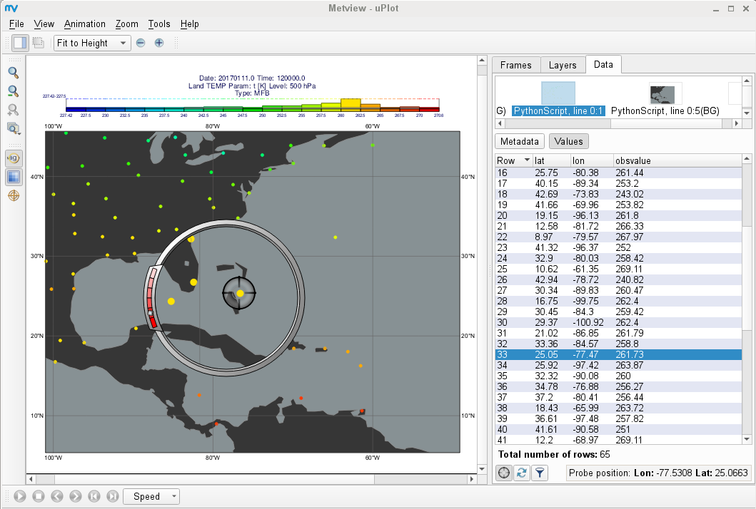
The data values can be inspected with the Cursor Data Tool (you can combine it with the Magnifier to see the fine details). Enable the sidebar of the Display Window with the

button and select the Data tab (and select the ‘vis_temp’ layer at the top if it is not yet selected). Now select the Metadata panel inside the tab. Here you will find some statistics about the data plotted and a histogram as well.

Now switch to the Values panel. This features a list showing all the plotted data. In the bottom-left corner click on the

button to activate the Data probe (this will appear in the plot). The probe is synchronised with the list. Try to drag it around in the plot, or change its position through the list. The Magnifier might help you position the Data probe more accurately.

Python Examples

There are a few Python examples in the folder for you to study. Open and run these scripts.

plot_map.py
	This is the Python code to generate the same plot as we did interactively above. The title and the symbol plotting value range are automatically computed from the actual data values. In the script we: used odb_visualiser() to generate the plot called odb_filter() (see odb_filter()) to extract additional data for the title used the values() function to access a given ODB column as a numpy array.
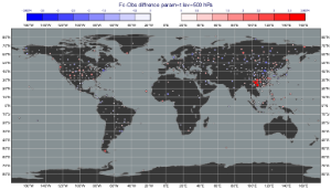
plot_diff.py
	This script computes the difference between the forecast fields stored in ‘fc.grib’ and our ODB observations. This is achieved by using the following steps: the ODB query is performed and the resulting data is converted into Geopoints the matching GRIB field is read and interpolated to the observation points the difference is computed between forecast and observation
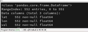
to_pandas.py
	This script shows how to convert an ODB into a Pandas dataframe with the to_dataframe() function.
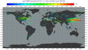
plot_wind.py
	This script shows how to plot wind data from ODB.

If you have extra time…

There are some other examples provided in the ‘4_odb’ folder (it is one level up from folder ‘main’).

Satellite radiances

Enter folder ‘radiance_map’.

“ASMUA.odb” stores AMSU-A brightness temperature observations. Use ‘tb_plot’ to visualise it and the other provided icons to customise the plot.

Scatterometer wind

Enter folder ‘scatterometer’.

‘SCATT.odb’ contains scatterometer data. The script ‘scatt,py’ extracts and plots scatterometer wind (ambiguous wind components) for a limited area and time period. Visualise the Python script and drop the provided ‘mslp.grib’ icon into the plot. This GRIB contains a mean sea level forecast valid at the same time as the observations.

Scatterplot

Enter folder ‘scatterplot’.

“ASMUA.odb” stores AMSU-A brightness temperature observations.

Visualise ‘scatter_plot’ and customise it with the provided Symbol Plotting icon. The plot you see is a scatterplot for the first guess departures (x axis) and analysis departures (y axis) for a given channel.

Visualise ‘bin_plot’ to get the binned version of the same data (as a heat map). Drop the provided Contouring, Cartesian View and Text Plotting icons into the plot to fully customise it.

Wind profiler

Enter folder ‘wind_profiler’.

‘PROF.odb’ contains wind profiler data. Use ‘profiler.mv’ to plot this data into a time-height diagram for a selected station.