Try this notebook in .

Filtering GRIB data

import time
import metview as mv

read() versus select()

Metview provides two ways to filter GRIB messages. Here is a quick comparison:

• read():

  • works with GRIB data from ECMWF’s archive, MARS

  • uses the same keywords as retrieve()

  • includes area cropping, spectral transforms and grid interpolation

  • has an equivalent icon in the graphical user interface, “GRIB Filter”

  • filtering may not be fully functional with non-MARS GRIB data

• select():

  • works with any GRIB data that ecCodes understands

  • uses ecCodes keys rather than MARS keywords

  • much faster than read() when called multiple times on the same Fieldset

  • no post-processing of data (use read() or regrid() separately for that)

  • only available from Python

filename = "data_fc.grib"
if mv.exist(filename):
    fs = mv.read(filename)
else:
    fs = mv.gallery.load_dataset(filename)

Inspecting the data

A separate notebook covers the details of inspecting GRIB data with Metview. Here we will use the methods to decide which fields to filter.

print(fs)

Fieldset (288 fields)

fs.describe()

parameter	typeOfLevel	level	date	time	step	paramId	class	stream	type	experimentVersionNumber
q	isobaricInhPa	100,250,...	20111215	0	0,6,...	133	od	oper	fc	0001
t	isobaricInhPa	100,250,...	20111215	0	0,6,...	130	od	oper	fc	0001
tp	surface	0	20111215	0	0,6,...	228	od	oper	fc	0001
u	isobaricInhPa	100,250,...	20111215	0	0,6,...	131	od	oper	fc	0001
v	isobaricInhPa	100,250,...	20111215	0	0,6,...	132	od	oper	fc	0001
z	isobaricInhPa	100,250,...	20111215	0	0,6,...	129	od	oper	fc	0001

OK, let’s select ‘t’ and have a closer look at what it has.

fs.describe('t')

shortName	t
name	Temperature
paramId	130
units	K
typeOfLevel	isobaricInhPa
level	100,250,300,500,700,850,1000
date	20111215
time	0
step	0,6,12,18,24,30,36,42
class	od
stream	oper
type	fc
experimentVersionNumber	0001

We have 8 forecast steps over 7 levels. We will make three selections:

• temperature at all fc steps for one level

• temperature at all fc steps for three levels

• temperature at two fc steps and three levels for a specific date

Filtering with read()

# temperature at all fc steps for one level
t_one = mv.read(data=fs, param='t', levelist=500)
t_one.ls()

	centre	shortName	typeOfLevel	level	dataDate	dataTime	stepRange	dataType	gridType
Message
0	ecmf	t	isobaricInhPa	500	20111215	0	0	fc	regular_ll
1	ecmf	t	isobaricInhPa	500	20111215	0	6	fc	regular_ll
2	ecmf	t	isobaricInhPa	500	20111215	0	12	fc	regular_ll
3	ecmf	t	isobaricInhPa	500	20111215	0	18	fc	regular_ll
4	ecmf	t	isobaricInhPa	500	20111215	0	24	fc	regular_ll
5	ecmf	t	isobaricInhPa	500	20111215	0	30	fc	regular_ll
6	ecmf	t	isobaricInhPa	500	20111215	0	36	fc	regular_ll
7	ecmf	t	isobaricInhPa	500	20111215	0	42	fc	regular_ll

# temperature at all fc steps for three levels
t_three = mv.read(data=fs, param='t', levelist=[100, 300, 500])
t_three.ls()

	centre	shortName	typeOfLevel	level	dataDate	dataTime	stepRange	dataType	gridType
Message
0	ecmf	t	isobaricInhPa	500	20111215	0	0	fc	regular_ll
1	ecmf	t	isobaricInhPa	300	20111215	0	0	fc	regular_ll
2	ecmf	t	isobaricInhPa	100	20111215	0	0	fc	regular_ll
3	ecmf	t	isobaricInhPa	500	20111215	0	6	fc	regular_ll
4	ecmf	t	isobaricInhPa	300	20111215	0	6	fc	regular_ll
5	ecmf	t	isobaricInhPa	100	20111215	0	6	fc	regular_ll
6	ecmf	t	isobaricInhPa	500	20111215	0	12	fc	regular_ll
7	ecmf	t	isobaricInhPa	300	20111215	0	12	fc	regular_ll
8	ecmf	t	isobaricInhPa	100	20111215	0	12	fc	regular_ll
9	ecmf	t	isobaricInhPa	500	20111215	0	18	fc	regular_ll
10	ecmf	t	isobaricInhPa	300	20111215	0	18	fc	regular_ll
11	ecmf	t	isobaricInhPa	100	20111215	0	18	fc	regular_ll
12	ecmf	t	isobaricInhPa	500	20111215	0	24	fc	regular_ll
13	ecmf	t	isobaricInhPa	300	20111215	0	24	fc	regular_ll
14	ecmf	t	isobaricInhPa	100	20111215	0	24	fc	regular_ll
15	ecmf	t	isobaricInhPa	500	20111215	0	30	fc	regular_ll
16	ecmf	t	isobaricInhPa	300	20111215	0	30	fc	regular_ll
17	ecmf	t	isobaricInhPa	100	20111215	0	30	fc	regular_ll
18	ecmf	t	isobaricInhPa	500	20111215	0	36	fc	regular_ll
19	ecmf	t	isobaricInhPa	300	20111215	0	36	fc	regular_ll
20	ecmf	t	isobaricInhPa	100	20111215	0	36	fc	regular_ll
21	ecmf	t	isobaricInhPa	500	20111215	0	42	fc	regular_ll
22	ecmf	t	isobaricInhPa	300	20111215	0	42	fc	regular_ll
23	ecmf	t	isobaricInhPa	100	20111215	0	42	fc	regular_ll

# temperature at two fc steps and three levels for a specific date
t_date = mv.read(data=fs, param='t', levelist=[100, 300, 500], step=[6, 24], date=20111215)
t_date.ls()

	centre	shortName	typeOfLevel	level	dataDate	dataTime	stepRange	dataType	gridType
Message
0	ecmf	t	isobaricInhPa	500	20111215	0	6	fc	regular_ll
1	ecmf	t	isobaricInhPa	300	20111215	0	6	fc	regular_ll
2	ecmf	t	isobaricInhPa	100	20111215	0	6	fc	regular_ll
3	ecmf	t	isobaricInhPa	500	20111215	0	24	fc	regular_ll
4	ecmf	t	isobaricInhPa	300	20111215	0	24	fc	regular_ll
5	ecmf	t	isobaricInhPa	100	20111215	0	24	fc	regular_ll

Filtering with select()

# temperature at all fc steps for one level
t_one = fs.select(shortName='t', level=500)
t_one.ls()

	centre	shortName	typeOfLevel	level	dataDate	dataTime	stepRange	dataType	gridType
Message
0	ecmf	t	isobaricInhPa	500	20111215	0	0	fc	regular_ll
1	ecmf	t	isobaricInhPa	500	20111215	0	6	fc	regular_ll
2	ecmf	t	isobaricInhPa	500	20111215	0	12	fc	regular_ll
3	ecmf	t	isobaricInhPa	500	20111215	0	18	fc	regular_ll
4	ecmf	t	isobaricInhPa	500	20111215	0	24	fc	regular_ll
5	ecmf	t	isobaricInhPa	500	20111215	0	30	fc	regular_ll
6	ecmf	t	isobaricInhPa	500	20111215	0	36	fc	regular_ll
7	ecmf	t	isobaricInhPa	500	20111215	0	42	fc	regular_ll

# temperature at all fc steps for three levels
# note that this example shows that select() performs some re-ordering of
# the fields for efficiency of filtering - compare with the equivalent read()
# example in the above section
t_three = fs.select(shortName='t', level=[100, 300, 500])
t_three.ls()

	centre	shortName	typeOfLevel	level	dataDate	dataTime	stepRange	dataType	gridType
Message
0	ecmf	t	isobaricInhPa	100	20111215	0	0	fc	regular_ll
1	ecmf	t	isobaricInhPa	300	20111215	0	0	fc	regular_ll
2	ecmf	t	isobaricInhPa	500	20111215	0	0	fc	regular_ll
3	ecmf	t	isobaricInhPa	100	20111215	0	6	fc	regular_ll
4	ecmf	t	isobaricInhPa	300	20111215	0	6	fc	regular_ll
5	ecmf	t	isobaricInhPa	500	20111215	0	6	fc	regular_ll
6	ecmf	t	isobaricInhPa	100	20111215	0	12	fc	regular_ll
7	ecmf	t	isobaricInhPa	300	20111215	0	12	fc	regular_ll
8	ecmf	t	isobaricInhPa	500	20111215	0	12	fc	regular_ll
9	ecmf	t	isobaricInhPa	100	20111215	0	18	fc	regular_ll
10	ecmf	t	isobaricInhPa	300	20111215	0	18	fc	regular_ll
11	ecmf	t	isobaricInhPa	500	20111215	0	18	fc	regular_ll
12	ecmf	t	isobaricInhPa	100	20111215	0	24	fc	regular_ll
13	ecmf	t	isobaricInhPa	300	20111215	0	24	fc	regular_ll
14	ecmf	t	isobaricInhPa	500	20111215	0	24	fc	regular_ll
15	ecmf	t	isobaricInhPa	100	20111215	0	30	fc	regular_ll
16	ecmf	t	isobaricInhPa	300	20111215	0	30	fc	regular_ll
17	ecmf	t	isobaricInhPa	500	20111215	0	30	fc	regular_ll
18	ecmf	t	isobaricInhPa	100	20111215	0	36	fc	regular_ll
19	ecmf	t	isobaricInhPa	300	20111215	0	36	fc	regular_ll
20	ecmf	t	isobaricInhPa	500	20111215	0	36	fc	regular_ll
21	ecmf	t	isobaricInhPa	100	20111215	0	42	fc	regular_ll
22	ecmf	t	isobaricInhPa	300	20111215	0	42	fc	regular_ll
23	ecmf	t	isobaricInhPa	500	20111215	0	42	fc	regular_ll

# temperature at two fc steps and three levels for a specific date
t_date = fs.select(shortName='t', level=[100, 300, 500], step=[6, 24], date=20111215)
t_date.ls()

	centre	shortName	typeOfLevel	level	dataDate	dataTime	stepRange	dataType	gridType
Message
0	ecmf	t	isobaricInhPa	100	20111215	0	6	fc	regular_ll
1	ecmf	t	isobaricInhPa	300	20111215	0	6	fc	regular_ll
2	ecmf	t	isobaricInhPa	500	20111215	0	6	fc	regular_ll
3	ecmf	t	isobaricInhPa	100	20111215	0	24	fc	regular_ll
4	ecmf	t	isobaricInhPa	300	20111215	0	24	fc	regular_ll
5	ecmf	t	isobaricInhPa	500	20111215	0	24	fc	regular_ll

# alternative: specify date using datetime
import datetime
t_date = fs.select(shortName='t', level=[100, 300, 500], step=[6, 24], date=datetime.datetime(2011, 12, 15, 0, 0))
t_date.ls()

	centre	shortName	typeOfLevel	level	dataDate	dataTime	stepRange	dataType	gridType
Message
0	ecmf	t	isobaricInhPa	100	20111215	0	6	fc	regular_ll
1	ecmf	t	isobaricInhPa	300	20111215	0	6	fc	regular_ll
2	ecmf	t	isobaricInhPa	500	20111215	0	6	fc	regular_ll
3	ecmf	t	isobaricInhPa	100	20111215	0	24	fc	regular_ll
4	ecmf	t	isobaricInhPa	300	20111215	0	24	fc	regular_ll
5	ecmf	t	isobaricInhPa	500	20111215	0	24	fc	regular_ll

Performance

Now we will compare the performance of these two methods and see how they differ when called multiple times on the same data. Imagine that we will want to compute a temporal mean for each level. To do that, we will loop over the levels and select all the forecast steps for each. We will enhance that code by adding timings, and by running the code multiple times, each time taking one more level into account.

def filter_n_times(n, use_select):
    levs = all_levels[0:n+1]
    for lev in levs:
        if use_select:
            a = fs.select(shortName='t', level=lev).count()
        else:
            a = mv.read(data=fs, param='t', levelist=lev).count()


# find the list of all levels
t_one_step = fs.select(shortName='t', step=0)
all_levels = t_one_step.grib_get_double('level')
num_levels = len(all_levels)

nlevs = []
times_read = []
times_select = []

for n in range(1, num_levels+1):
    nlevs.append(n)
    time1 = time.perf_counter()
    filter_n_times(n, use_select=True)
    timediff = time.perf_counter() - time1
    times_select.append(timediff)

    time1 = time.perf_counter()
    filter_n_times(n, use_select=False)
    timediff = time.perf_counter() - time1
    times_read.append(timediff)

import matplotlib.pyplot as plt

plt.plot(nlevs, times_select, label="select")
plt.plot(nlevs, times_read, label="read")
plt.xlabel("Number of filters")
plt.ylabel("time (s)")
plt.legend(loc='upper left')
plt.title('select vs read - small values mean faster')

plt.show()

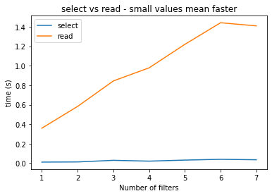
The performance differences are due to the fact that select() caches its Fieldset indexes so that further filtering on the same Fieldset should be faster.