Try this notebook in ![]() .
.
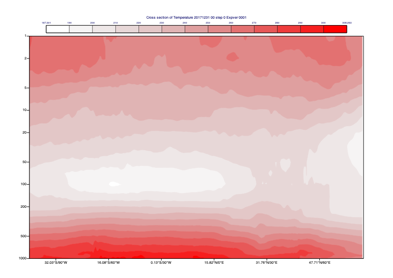
Cross Section example using reanalysis GRIB data from CDS
Demonstrates how to use Metview to compute and plot a vertical cross section of an ERA5 GRIB file retrieved from the Climate Data Store (CDS).
[7]:
import metview as mv
import cdsapi
Retrieve ERA5 temperature data in GRIB format using the CDS API (access needs to be set up first). If you do not have access to the CDS-API then initialise variable use_cds = False. A copy of the data is provided on disk.
[8]:
use_cds = False
filename = "era5_temp_from_cds.grib"
if use_cds:
    c = cdsapi.Client()
    c.retrieve("reanalysis-era5-pressure-levels",
        {
          "variable": "temperature",
          "pressure_level":['1','2','3','5','7','10','20','30','50','70','100','150',
                        '200','250','300','400','500','600','700','800','850',
                        '900','925','950','1000'
                      ],
          "product_type": "reanalysis",
          "date": "20171231",
          "time": "00:00",
          "format": "grib"
        },
        filename)
    fs = mv.read(filename)
else:
    if mv.exist(filename):
        fs = mv.read(filename)
    else:
        fs = mv.gallery.load_dataset(filename)
Metview reads the GRIB data into its Fieldset class.
Define an mxsectview(), setting parameters required for the cross section computation and visualisation, including a geographical line along which a cross section of the data is computed (remember that the data consists of a number of vertical levels).
[9]:
xsection_view = mv.mxsectview(
    vertical_scaling = "log",
    bottom_level     = 1000.0,
    top_level        = 1,
    line             = [-40, -105, 61, 85] #lat,lon,lat,lon
)
Sets up an mcont(), which provides much flexibility in choosing how to display the output data. It controls features such as isolines, shading and colour schemes.
[10]:
shading = mv.mcont(
    legend                         = "on",
    contour                        = "off",
    contour_level_count            = 12,
    contour_label                  = "off",
    contour_shade                  = "on",
    contour_shade_method           = "area_fill",
    contour_shade_max_level_colour = "red",
    contour_shade_min_level_colour = "white"
)
To plot this, we first need to tell Metview to send the plot to Jupyter.
[11]:
mv.setoutput('jupyter')
Plot the data into the Cross Section View with a customized contouring style.
[12]:
mv.plot(xsection_view, fs, shading)
[12]:
[ ]: