Try this notebook in .

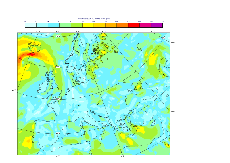
Retrieving netCDF data from the CDS and plotting it with Metview

Demonstrates how to retrieve netCDF data from the Climate Data Store (CDS) and visualise it with Metview using automatic styling and a polar stereographic projection.

import metview as mv
import cdsapi

Retrieves ERA5 instantaneous 10 metre wind gust data in netCDF format using the CDS API (access needs to be set up first). If you do not have access to the CDS-API then initialise variable use_cds = False. A copy of the data is provided on disk.

use_cds = False
filename = "wgust_era5.nc"
if use_cds:
    c = cdsapi.Client()
    c.retrieve("reanalysis-era5-pressure-levels",
               {
                   "variable": "instantaneous_10m_wind_gust",
                   "product_type": "reanalysis",
                   "year": "2011",
                   "month": "08",
                   "day": "01",
                   "time": "00:00",
                   "format": "netcdf"
               },
               filename)
    ncdata = mv.read(filename)
else:
    if mv.exist(filename):
        ncdata = mv.read(filename)
    else:
        ncdata = mv.gallery.load_dataset(filename)

Defines the netCDF variable to be visualised using netcdf_visualiser().

ncvis = mv.netcdf_visualiser(
    netcdf_plot_type          = "geo_matrix",
    netcdf_data               = ncdata,
    netcdf_latitude_variable  = "latitude",
    netcdf_longitude_variable = "longitude",
    netcdf_value_variable     = "i10fg"
    )

Defines a geoview() to customise parameters like map projection and geographical area.

geoview = mv.geoview(
    map_projection      = "polar_stereographic",
    map_area_definition = "corners",
    area                = [33,-13,49,64]    #[S,W,N,E]
    )

Sets up the contouring style with mcont(), which provides much flexibility in choosing how to display the output data. It controls features such as isolines, shading and colour schemes. Here, we use a Magics automatic styling.

cont = mv.mcont(
    contour_automatic_setting = "style_name",
    contour_style_name        = "sh_all_f03t70_beauf",
    legend                    = "on"
    )

To plot this, we first need to tell Metview to send the plot to Jupyter.

mv.setoutput('jupyter')

Plot the netcdf data into the customised view and contouring style.

mv.plot(geoview, ncvis, cont)