Try this notebook in ![]() .
.
Inspecting GRIB data
When running Metview through its graphical user interface, the easiest way to inspect a GRIB file is to right-click on it and choose ‘examine’ from the context menu. Similar functionality is available from the command line: “metview -e /path/to/grib/file”.
This notebook shows how to inspect GRIB data from within a Python environment. Note that filtering, processing and visualising data is covered in other notebooks and gallery examples.
[1]:
import metview as mv
[2]:
filename = "data_fc.grib"
if mv.exist(filename):
    fs = mv.read(filename)
else:
    fs = mv.gallery.load_dataset(filename)
Data overview
In Metview, GRIB data is represented by a Fieldset object. Many Metview operations generate GRIB data, we can retrieve it from MARS, or we can load it directly from disk.
GRIB files are composed of messages, one for each field. The describe() method groups the GRIB messages by parameter and gives a summary for quick inspection. Here we will see that the Fieldset contains parameters q,t,u,v,z for multiple vertical levels, and tp at surface level at various forecast steps. We will see in a moment what these parameters actually are in case you’re not familiar with the letters!
[3]:
fs.describe()
[3]:
| parameter | typeOfLevel | level | date | time | step | paramId | class | stream | type | experimentVersionNumber |
|---|---|---|---|---|---|---|---|---|---|---|
| q | isobaricInhPa | 100,250,... | 20111215 | 0 | 0,6,... | 133 | od | oper | fc | 0001 |
| t | isobaricInhPa | 100,250,... | 20111215 | 0 | 0,6,... | 130 | od | oper | fc | 0001 |
| tp | surface | 0 | 20111215 | 0 | 0,6,... | 228 | od | oper | fc | 0001 |
| u | isobaricInhPa | 100,250,... | 20111215 | 0 | 0,6,... | 131 | od | oper | fc | 0001 |
| v | isobaricInhPa | 100,250,... | 20111215 | 0 | 0,6,... | 132 | od | oper | fc | 0001 |
| z | isobaricInhPa | 100,250,... | 20111215 | 0 | 0,6,... | 129 | od | oper | fc | 0001 |
We can look a bit deeper into each parameter via its shortName, for example, temperature:
[4]:
fs.describe("t")
[4]:
| shortName | t |
|---|---|
| paramId | 130 |
| typeOfLevel | isobaricInhPa |
| level | 100,250,300,500,700,850,1000 |
| date | 20111215 |
| time | 0 |
| step | 0,6,12,18,24,30,36,42 |
| class | od |
| stream | oper |
| type | fc |
| experimentVersionNumber | 0001 |
Note that the data do not necessarily form a complete hypercube - this summary lists all the values for each ‘dimension’, but it is not necessarily the case that, for example, all the steps exist for all the levels.
We can also specify the parameter via its numeric paramId, for example, total precipitation:
[5]:
fs.describe(228)
[5]:
| shortName | tp |
|---|---|
| paramId | 228 |
| typeOfLevel | surface |
| level | 0 |
| date | 20111215 |
| time | 0 |
| step | 0,6,12,18,24,30,36,42 |
| class | od |
| stream | oper |
| type | fc |
| experimentVersionNumber | 0001 |
Data table
fs is a Fieldset object representing the GRIB file. It is essentially a list of GRIB messages. The ls() method displays information on a per-message basis. We can call it with the whole Fieldset, but that gives us a very long listing! So let’s call it on the first 10 fields using Python’s ‘slice’ operator:
[6]:
fs[:10].ls()
[6]:
| centre | shortName | typeOfLevel | level | dataDate | dataTime | stepRange | dataType | gridType | |
|---|---|---|---|---|---|---|---|---|---|
| Message | |||||||||
| 0 | ecmf | t | isobaricInhPa | 1000 | 20111215 | 0 | 0 | fc | regular_ll |
| 1 | ecmf | z | isobaricInhPa | 1000 | 20111215 | 0 | 0 | fc | regular_ll |
| 2 | ecmf | u | isobaricInhPa | 1000 | 20111215 | 0 | 0 | fc | regular_ll |
| 3 | ecmf | v | isobaricInhPa | 1000 | 20111215 | 0 | 0 | fc | regular_ll |
| 4 | ecmf | q | isobaricInhPa | 1000 | 20111215 | 0 | 0 | fc | regular_ll |
| 5 | ecmf | t | isobaricInhPa | 850 | 20111215 | 0 | 0 | fc | regular_ll |
| 6 | ecmf | z | isobaricInhPa | 850 | 20111215 | 0 | 0 | fc | regular_ll |
| 7 | ecmf | u | isobaricInhPa | 850 | 20111215 | 0 | 0 | fc | regular_ll |
| 8 | ecmf | v | isobaricInhPa | 850 | 20111215 | 0 | 0 | fc | regular_ll |
| 9 | ecmf | q | isobaricInhPa | 850 | 20111215 | 0 | 0 | fc | regular_ll |
We can select a different range of fields and add extra ecCodes keys to get more information:
[7]:
fs[210:220].ls(extra_keys=['name', 'units'])
[7]:
| centre | shortName | typeOfLevel | level | dataDate | dataTime | stepRange | dataType | gridType | name | units | |
|---|---|---|---|---|---|---|---|---|---|---|---|
| Message | |||||||||||
| 0 | ecmf | t | isobaricInhPa | 1000 | 20111215 | 0 | 36 | fc | regular_ll | Temperature | K |
| 1 | ecmf | z | isobaricInhPa | 1000 | 20111215 | 0 | 36 | fc | regular_ll | Geopotential | m**2 s**-2 |
| 2 | ecmf | u | isobaricInhPa | 1000 | 20111215 | 0 | 36 | fc | regular_ll | U component of wind | m s**-1 |
| 3 | ecmf | v | isobaricInhPa | 1000 | 20111215 | 0 | 36 | fc | regular_ll | V component of wind | m s**-1 |
| 4 | ecmf | q | isobaricInhPa | 1000 | 20111215 | 0 | 36 | fc | regular_ll | Specific humidity | kg kg**-1 |
| 5 | ecmf | t | isobaricInhPa | 850 | 20111215 | 0 | 36 | fc | regular_ll | Temperature | K |
| 6 | ecmf | z | isobaricInhPa | 850 | 20111215 | 0 | 36 | fc | regular_ll | Geopotential | m**2 s**-2 |
| 7 | ecmf | u | isobaricInhPa | 850 | 20111215 | 0 | 36 | fc | regular_ll | U component of wind | m s**-1 |
| 8 | ecmf | v | isobaricInhPa | 850 | 20111215 | 0 | 36 | fc | regular_ll | V component of wind | m s**-1 |
| 9 | ecmf | q | isobaricInhPa | 850 | 20111215 | 0 | 36 | fc | regular_ll | Specific humidity | kg kg**-1 |
We can add some keys that compute statistics per field (this will take longer, as the values will be decoded and the statistics computed - they are not stored in the GRIB header).
[8]:
fs[210:220].ls(extra_keys=['min', 'max'])
[8]:
| centre | shortName | typeOfLevel | level | dataDate | dataTime | stepRange | dataType | gridType | min | max | |
|---|---|---|---|---|---|---|---|---|---|---|---|
| Message | |||||||||||
| 0 | ecmf | t | isobaricInhPa | 1000 | 20111215 | 0 | 36 | fc | regular_ll | 250.973 | 312.973 |
| 1 | ecmf | z | isobaricInhPa | 1000 | 20111215 | 0 | 36 | fc | regular_ll | -2506.38 | 3061.62 |
| 2 | ecmf | u | isobaricInhPa | 1000 | 20111215 | 0 | 36 | fc | regular_ll | -14.0416 | 19.7084 |
| 3 | ecmf | v | isobaricInhPa | 1000 | 20111215 | 0 | 36 | fc | regular_ll | -16.6044 | 19.3956 |
| 4 | ecmf | q | isobaricInhPa | 1000 | 20111215 | 0 | 36 | fc | regular_ll | 8.95455e-05 | 0.0198649 |
| 5 | ecmf | t | isobaricInhPa | 850 | 20111215 | 0 | 36 | fc | regular_ll | 245.139 | 302.639 |
| 6 | ecmf | z | isobaricInhPa | 850 | 20111215 | 0 | 36 | fc | regular_ll | 10344.5 | 16136.5 |
| 7 | ecmf | u | isobaricInhPa | 850 | 20111215 | 0 | 36 | fc | regular_ll | -16.2513 | 26.9987 |
| 8 | ecmf | v | isobaricInhPa | 850 | 20111215 | 0 | 36 | fc | regular_ll | -21.4716 | 25.5284 |
| 9 | ecmf | q | isobaricInhPa | 850 | 20111215 | 0 | 36 | fc | regular_ll | 8.98526e-05 | 0.0155317 |
We can also use type qualifiers (s=string, l=long, d=double) to give more control over how the keys are displayed:
[10]:
fs[210:220].ls(extra_keys=['centre:l'])
[10]:
| centre | shortName | typeOfLevel | level | dataDate | dataTime | stepRange | dataType | gridType | centre:l | |
|---|---|---|---|---|---|---|---|---|---|---|
| Message | ||||||||||
| 0 | ecmf | t | isobaricInhPa | 1000 | 20111215 | 0 | 36 | fc | regular_ll | 98.0 |
| 1 | ecmf | z | isobaricInhPa | 1000 | 20111215 | 0 | 36 | fc | regular_ll | 98.0 |
| 2 | ecmf | u | isobaricInhPa | 1000 | 20111215 | 0 | 36 | fc | regular_ll | 98.0 |
| 3 | ecmf | v | isobaricInhPa | 1000 | 20111215 | 0 | 36 | fc | regular_ll | 98.0 |
| 4 | ecmf | q | isobaricInhPa | 1000 | 20111215 | 0 | 36 | fc | regular_ll | 98.0 |
| 5 | ecmf | t | isobaricInhPa | 850 | 20111215 | 0 | 36 | fc | regular_ll | 98.0 |
| 6 | ecmf | z | isobaricInhPa | 850 | 20111215 | 0 | 36 | fc | regular_ll | 98.0 |
| 7 | ecmf | u | isobaricInhPa | 850 | 20111215 | 0 | 36 | fc | regular_ll | 98.0 |
| 8 | ecmf | v | isobaricInhPa | 850 | 20111215 | 0 | 36 | fc | regular_ll | 98.0 |
| 9 | ecmf | q | isobaricInhPa | 850 | 20111215 | 0 | 36 | fc | regular_ll | 98.0 |
We can add a filter to show only those messages whose keys match all the given conditions. Note that these must be valid ecCodes keys - ‘shortName’ or ‘paramId’ can be used for the parameter, but ‘param’ cannot, since it is not a key. Keys do not need to be displayed in order to be used as a filter.
[27]:
fs.ls(filter={'shortName':'t', 'step':6, 'centre:s':'ecmf'})
[27]:
| centre | shortName | typeOfLevel | level | dataDate | dataTime | stepRange | dataType | gridType | |
|---|---|---|---|---|---|---|---|---|---|
| Message | |||||||||
| 35 | ecmf | t | isobaricInhPa | 1000 | 20111215 | 0 | 6 | fc | regular_ll |
| 40 | ecmf | t | isobaricInhPa | 850 | 20111215 | 0 | 6 | fc | regular_ll |
| 45 | ecmf | t | isobaricInhPa | 700 | 20111215 | 0 | 6 | fc | regular_ll |
| 50 | ecmf | t | isobaricInhPa | 500 | 20111215 | 0 | 6 | fc | regular_ll |
| 55 | ecmf | t | isobaricInhPa | 300 | 20111215 | 0 | 6 | fc | regular_ll |
| 60 | ecmf | t | isobaricInhPa | 250 | 20111215 | 0 | 6 | fc | regular_ll |
| 65 | ecmf | t | isobaricInhPa | 100 | 20111215 | 0 | 6 | fc | regular_ll |
Note that the output from ls() is a pandas dataframe, allowing further manipulation:
[12]:
p = fs[:10].ls()
print(type(p))
print(p.columns)
print(p['shortName'])
<class 'pandas.core.frame.DataFrame'>
Index(['centre', 'shortName', 'typeOfLevel', 'level', 'dataDate', 'dataTime',
       'stepRange', 'dataType', 'gridType'],
      dtype='object')
Message
0    t
1    z
2    u
3    v
4    q
5    t
6    z
7    u
8    v
9    q
Name: shortName, dtype: object
Getting more specific keys
To extract just the keys you want from the GRIB fields, use grib_get_long(), grib_get_double() and grib_get_string() to extract single keys, and grib_get() for multiple keys. These examples show how.
[13]:
fs[:5].grib_get_string('centre')
[13]:
['ecmf', 'ecmf', 'ecmf', 'ecmf', 'ecmf']
[15]:
fs[:5].grib_get_long('centre')
[15]:
[98.0, 98.0, 98.0, 98.0, 98.0]
[20]:
fs[43:48].grib_get_double('level')
[20]:
[850.0, 850.0, 700.0, 700.0, 700.0]
When extracting mutliple keys, it is more efficient to use grib_get() to get them all in one go:
[23]:
fs[43:48].grib_get(['centre', 'step', 'level'])
[23]:
[['ecmf', '6', '850'],
 ['ecmf', '6', '850'],
 ['ecmf', '6', '700'],
 ['ecmf', '6', '700'],
 ['ecmf', '6', '700']]
Since the grib_get() method does not specify a type for each key, we can add :l, :d or :s to each one:
[25]:
fs[43:48].grib_get(['centre:l', 'step', 'level'])
[25]:
[[98.0, '6', '850'],
 [98.0, '6', '850'],
 [98.0, '6', '700'],
 [98.0, '6', '700'],
 [98.0, '6', '700']]
The above command will return a list per field. We can instead tell it to group the results by key:
[26]:
fs[43:48].grib_get(['centre:l', 'step', 'level'], 'key')
[26]:
[[98.0, 98.0, 98.0, 98.0, 98.0],
 ['6', '6', '6', '6', '6'],
 ['850', '850', '700', '700', '700']]
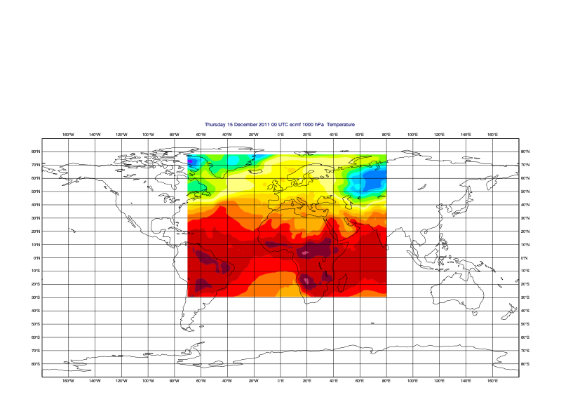
Quick plot
Let’s plot the first field to see the geographic extents of the data:
[34]:
mv.setoutput('jupyter')
mv.plot(fs[0], mv.mcont(contour_automatic_setting='ecmwf'))
[34]:
[ ]: