Version 5.17 Updates
Version 5.17.4
Installed as part of ecmwf-toolbox/2022.08.3.0 (Atos HPC, tag ‘new’)
At ECMWF:
Fixes:
Cross Section View: fixed issue where dropping a MARS Retrieval icon into the view produced an incorrect plot
Desktop: fixed issue where the icon search could crash
Version 5.17.3
Installed as part of ecmwf-toolbox/2022.08.2.0 (Atos HPC, tag ‘new’)
At ECMWF:
Fixes:
MARS client: updated client to allow retrieval of observations from the RDB
GRIB Filter: fixed issue where parameter order=’sorted’ incorrectly sorted by step
Bufr Picker: fixed issue where polar_vector output was not working
FLEXPART: fixed issue where shortName was wrongly changed from mdc to mdens in the GRIB results
Desktop: fixed issue where folder with broken link could be attempted to be opened
Version 5.17.2
Installed as part of ecmwf-toolbox/2022.08.1.0 (Atos HPC, tag ‘new’)
At ECMWF:
Fixes:
Meteogram module (
meteogram()) uses URL to retrieve charts from Bologna by defaultMeteogram module: fixed issue where the specified time was ignored and the meteogram for time 00UTC was always retrieved
FLEXPART: fixed paths to FLEXPART executable and resources at ECMWF
Macro: fixed issue in the
mask()function that caused an infinite loop if an area that straddled the date line was given
Version 5.17.0
Externally released on 2022-08-24
Became metview/new at ECMWF on 2022-08-24 (Linux desktops, ecgate, lxc, lxop, Cray HPC)
Installed as part of ecmwf-toolbox/2022.08.0.0 (Atos HPC)
At ECMWF:
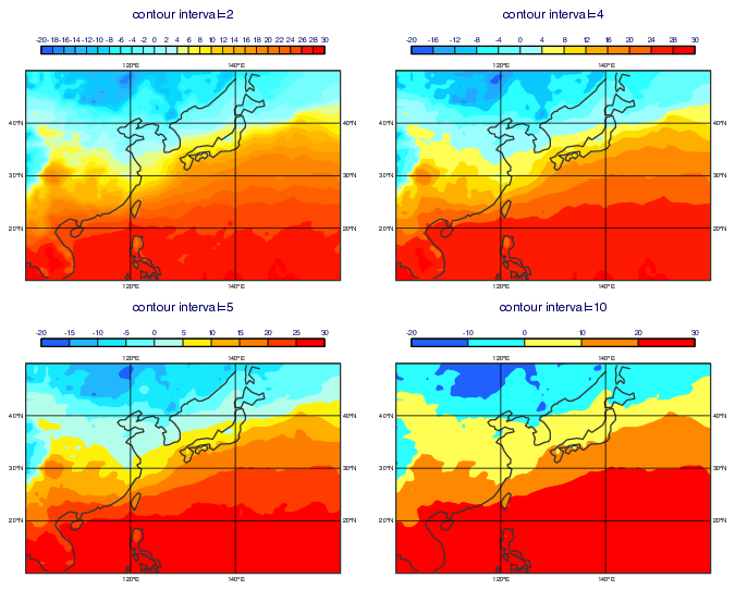
Plotting
mcont() can automatically adjust predefined palettes and user defined colour lists to the actual contour level values with the new contour_shade_colour_list_policy = “dynamic” option. It is also possible to reverse palettes and colour lists for plotting by setting contour_shade_colour_reverse_list to “on”. See the gallery example:
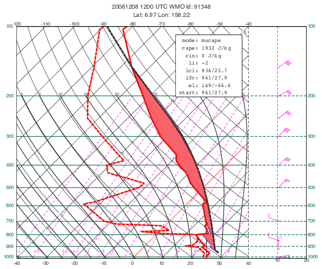
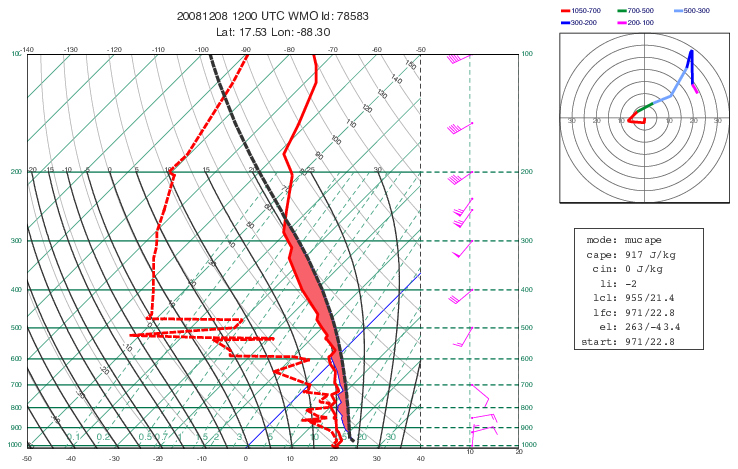
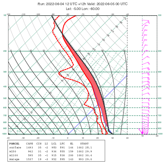
Thermo parcel path
The parcel computations have been revised and several new option were added:
lifted_condensation_level(): improved speed by using [Bolton1980] instead of an iterative process to compute the \(t_{LCL}\). Works now with ndarrays andFieldsetas input (previously only numbers were accepted).-
Algorithmic changes:
the equivalent potential temperature defining the pseudo-adiabatic path is now computed with formula (39) from [Bolton1980]
the LFC (Level of Free Convection) is now determined as the bottom pressure of the positive buoyancy area highest in the atmosphere. This results in improved CIN computation when there are multiple positive buoyancy areas above the LCL. In these situations the CIN was formerly underestimated.
the Lifted Index (LI) is now computed and added to the output
Interface changes:
the
optionsbecame keyword arguments. Previously they were specified as a dict as the last positional argument. The old interface still works for backwards compatibility. E.g.:# the new interface mv.thermo_parcel_path(prof, mode="surface", stop_at_el=False) # the old interface mv.thermo_parcel_path(prof, {"mode": "surface", "stop_at_el": False})
The computations can now use the virtual temperature correction, which is enabled by default. See the
virtualkey in theoptionsargument.The “most_unstable” mode was renamed “mucape”. The old name is still supported but deprecated.
The “mean_layer” mode was renamed “ml”. The old name is still supported but deprecated.
The “ml” start conditions are determined in a new way. Previously simply the mean values of temperature, dewpoint and pressure in the given layer were used. Now, the temperature is determined from the mean potential temperature, the dewpoint is the mean value in the layer and pressure is the surface pressure.
New start modes were added: “m50” and “ml100”. They are the variants of the “ml” mode with a fixed 50 hPa and 100 hPa bottom layer, respectively.
The size of the layer in “ml” and “mucape” mode can now be specified via the
layer_depthparameter.The default start conditions were changed to
mode= “mucape” withlayer_depth= 300. E.g.:# these calls are now equivalent mv.thermo_parcel_path(prof) mv.thermo_parcel_path(prof, mode="mucape", layer_depth=300)
Added new parameters
compute_topto control the computations and data extraction above the Equilibrium Level (EL)See the gallery example showcasing some of the new features:
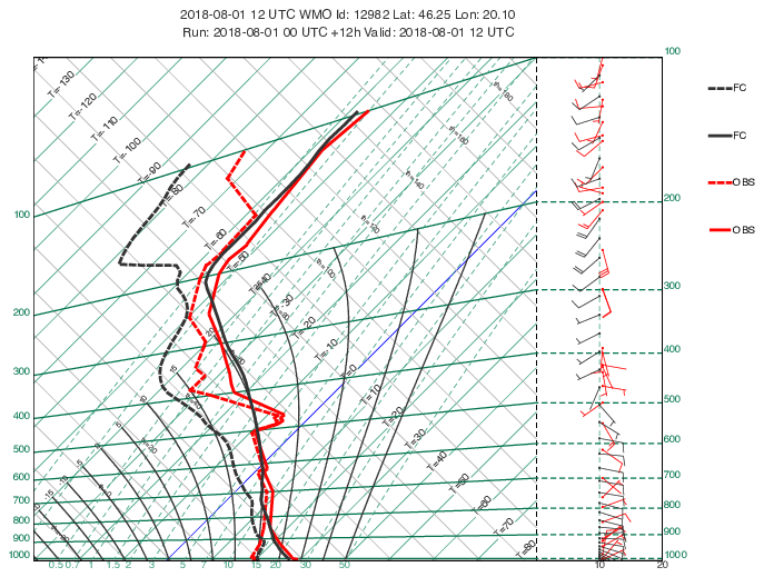
Thermo profile
Thermo Bufr: added new parameters to specify location by WMO name, WMO ident and WIGOS Station Identifier. See:
thermo_bufr()andthermoview().Improved error message when no BUFR message matching the required location and BUFR data subtype was found in input.
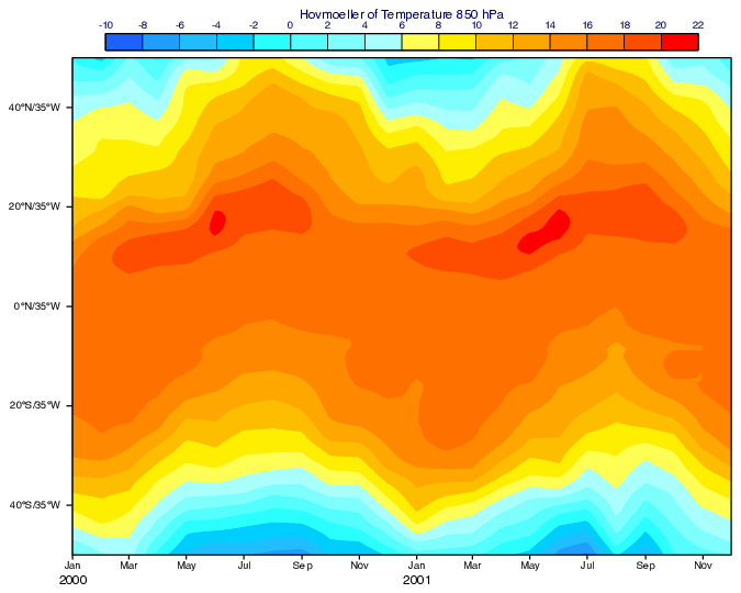
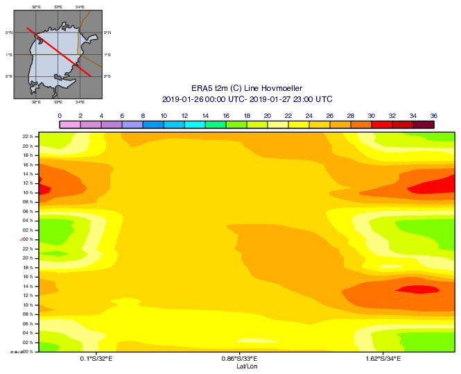
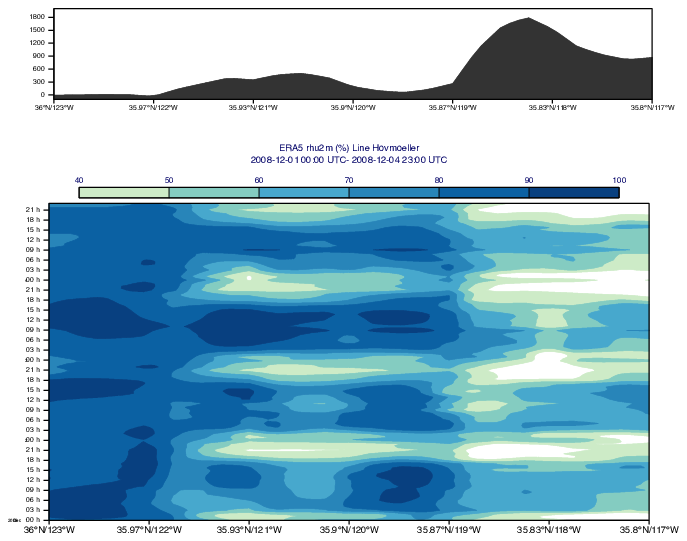
Hovmoller
Vertical Hovmoeller: added new parameters
use_fixed_surface_pressureandfixed_surface_pressureto use a fixed surface pressure value in the computations. These can be used when the input data is model level and the vertical axis is pressure (vertical_level_type= “pressure”). See:mhovmoellerview()andmhovmoeller_vertical().Line Hovmoeller: fixed issue when North and South coordinates of lines going from SW to NE were automatically swapped
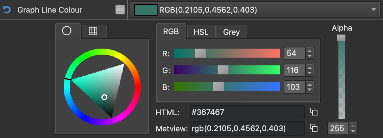
User interface
Colour editor: redesigned interface and added RGB, HSL and greyscale colour sliders
Desktop: added “Copy filesystem path” action to the context menu of the Breadcrumbs items
Contour icon editor: added option to show/hide filter options for palette chooser interface
Family icons: fixed issue when could not edit newly created family icons
Advanced search: fixed issue when search did not work with time period in Metview versions built with Qt >= 5.8.0
Advanced search: fixed issue when results from the last day of time period were excluded
Grib Examiner: fixed issue when the value of the mars.expver key was not shown in the Namespace dump
FLEXTRA/FLEXPART
flextra_prepare(): added parameterflextra_an_mars_classto control the MARS class of the analysis data retrieved whenflextra_prepare_modeis “period”. The possible values are “od” (operational analysis) and “ea” (ERA5).flextra_prepare(): fixed issue when settingflextra_prepare_modeto “period” caused an errorflexpart_prepare(): fixed issue when settingflexpart_prepare_modeto “period” caused an error
Macro/Python
mean()andsum(): added new parameterdimto restrict computations to a specific dimension ofFieldsetdata in python, e.g. compute an ensemble mean when multiple steps exist in the dataadded new function
pl_to_pl()to perform interpolation from pressure level GRIB fields onto a set of target pressure levelsimproved speed and reduced memory usage in many GRIB-related functions
added new function
static_stability()to compute the static stability. See the gallery example: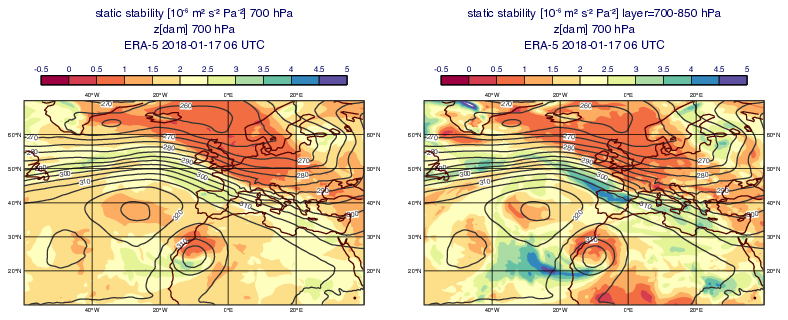
added new function
q_vector()to compute the Q-vector used in the quasi-geostrophic (QG) theory. See the gallery example: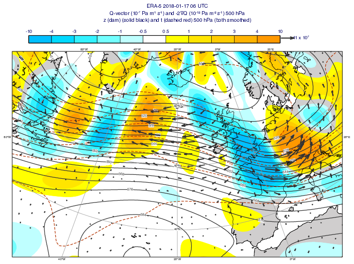
added new functions
smooth_n_point()andsmooth_gaussian()to perform spatial smoothing on fieldsets with lat-lon grids. See the gallery example: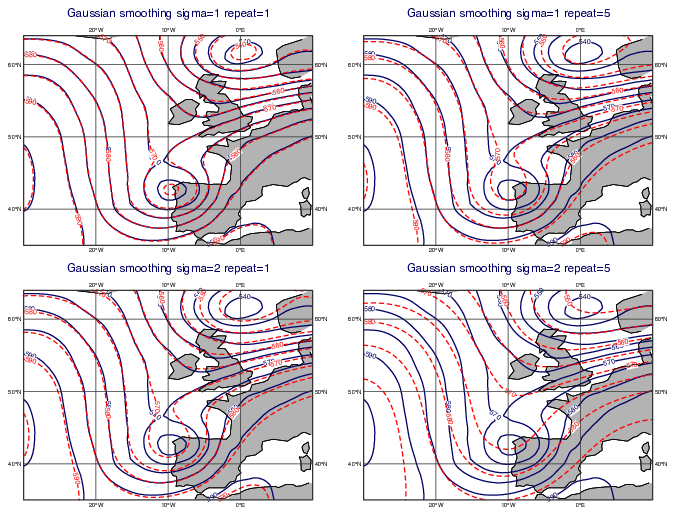
added new function
convolve()to perform spatial 2D convolution on fieldsets with lat-lon gridsadded new function
rms_a()to compute area-weighted root mean square for each field in a fieldsetadded new function
grib_indexes()to return GRIB message information for a Fieldsetgrib_set(): added new optionrepackto repack GRIB data. It is required to use when setting some ecCodes keys (e.g. packingType) involving properties of the packing algorithm.geostrophic_wind(): added new optioncoriolisto use a constant Coriolis parameter valuemvl_ml2hPa(): allowed to specify the target pressure levels as an ndarraydirection(): fixed issue when the ecCodes paramId in the resulting field was not set to 131 (=wind direction)fixed issue when using fields with mixed expver caused Metview to hang in cross section, average cross section, vertical profile and Hovmoeller computations and plotting
New Gallery Examples